PSTAT 100: Lecture 19
Clustering; Introduction to Missing Data
Clustering vs. Classification
The first topic of today’s lecture, clustering, is the unsupervised analog of classification.
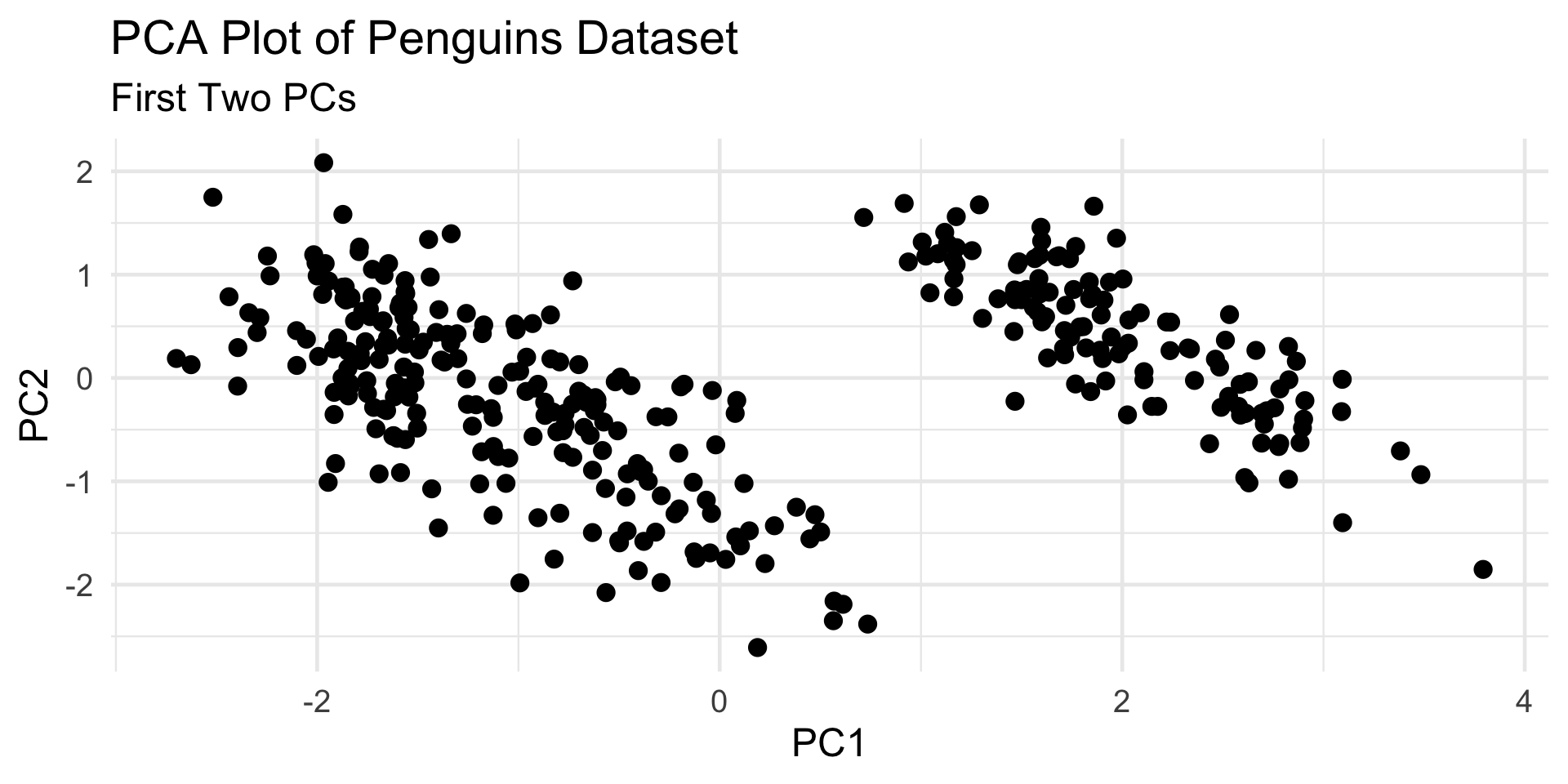
As an example, consider the following scatterplot of penguins Bill Lengths plotted against their Body Mass:
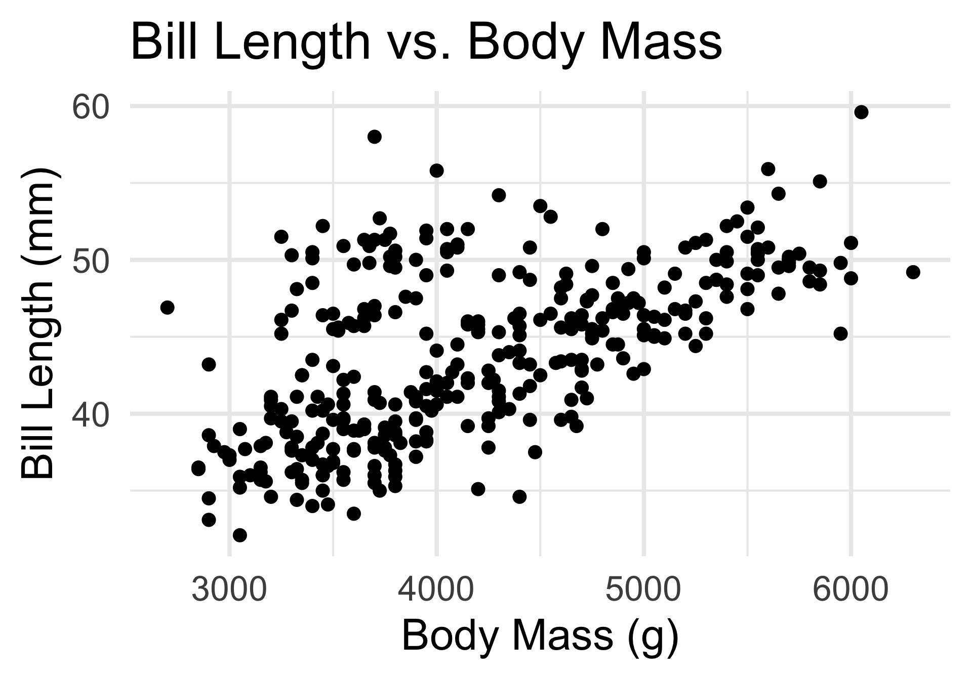
- Here’s a question: how many “groups” (clusters) of points do you see?
- Note that I’m not asking about the relationship between any two variables!
Clustering
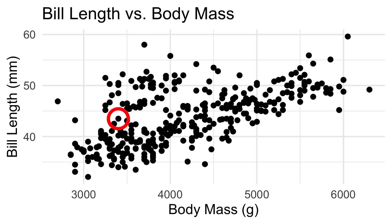
By eye, it looks like there are potentially two main clusters.
But the boundaries between these clusters are perhaps a bit “fuzzy”.
For example, which group should the circled point belong to?
Clustering
Subpopulations or Not
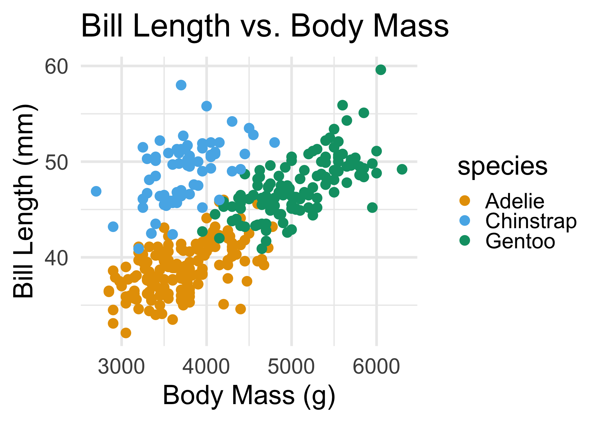
In this problem, there just so happened to exist three subpopulations in our data, and that this was what was driving our observations about clusters.
But clustering works just as well when there aren’t natural subpopulations in the data.
- For illustrative purposes, let’s stick with the penguins dataset and increase the number of variables we consider.
Penguins, Revisited
PCA
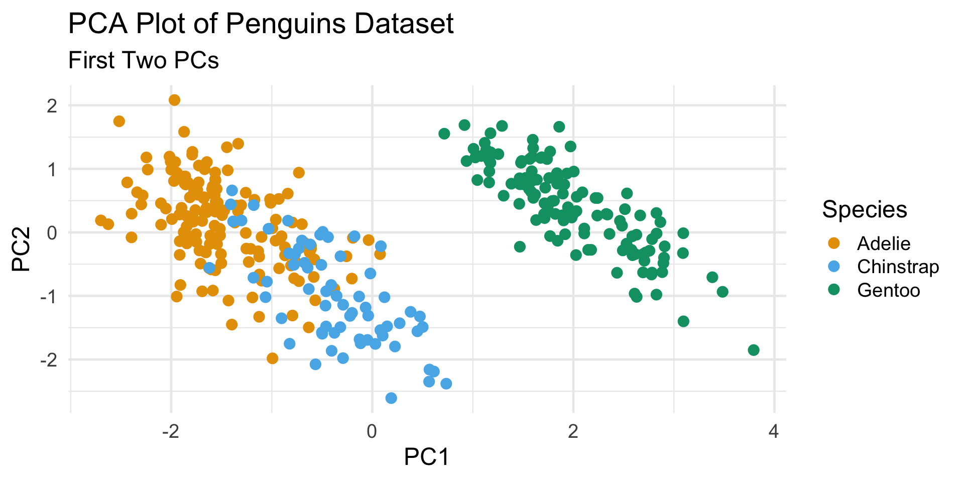
Even when there exist subpopulations, our clusters may not always reflect them (particularly if two or more subpopulations are very similar to one another).
In this way, we can perhaps think of clustering as identifying “inherent subpopulations” (like PCA uncovers “inherent dimensionality”)
Votes, Revisited
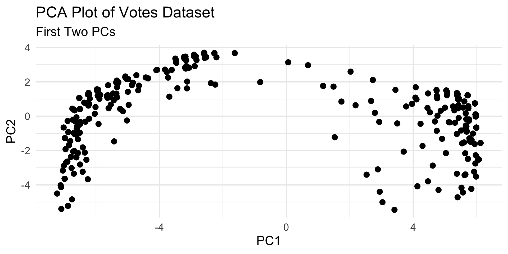
- How many clusters? Two? Three?
Votes, Revisited
Clustering
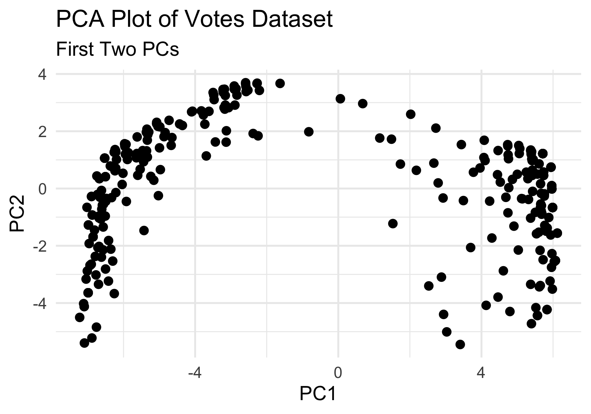
- Let’s say we believe there to be two clusters in our data.
- Even with that determination, there is still the question of where to place our cluster boundaries.
- So, let’s discuss some techniques for setting those.
K-Means Clustering
- One of the most widely-known clustering techniques is that of K-means.

Identify the cluster centroids by minimizing the variance within each cluster

Identify the cluster assignments by finding the shortest Euclidean distance to a centroid
K-Means Clustering
Votes Dataset
Code
set.seed(100)   ## for reproducibility

km_votes <- kmeans(votes_num, centers = 2)
prcomp(votes_num, scale. = TRUE)$x[,1:2] %>%
  data.frame() %>%
  mutate(kmeans_clust = factor(km_votes$cluster)) %>%
  ggplot(aes(x = PC1, y = PC2)) +
  geom_point(size = 3,
             aes(col = kmeans_clust)) +
  theme_minimal(base_size = 18) +
  ggtitle("PCA Plot of Votes Dataset",
          subtitle = "Clustered using K-Means") +
  scale_color_okabe_ito() +
  labs(col = "Cluster")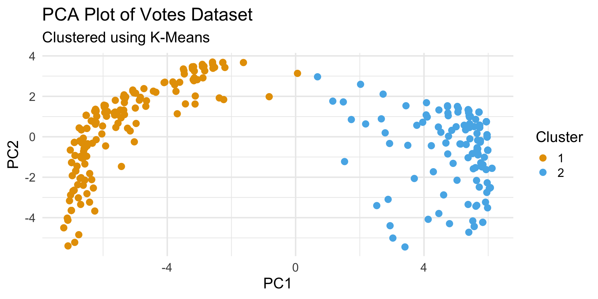
K-Means Clustering
Votes Dataset
K-Means Clustering
Votes Dataset
- Also, we can examine the one person whose party affiliation is missing from the original dataset:
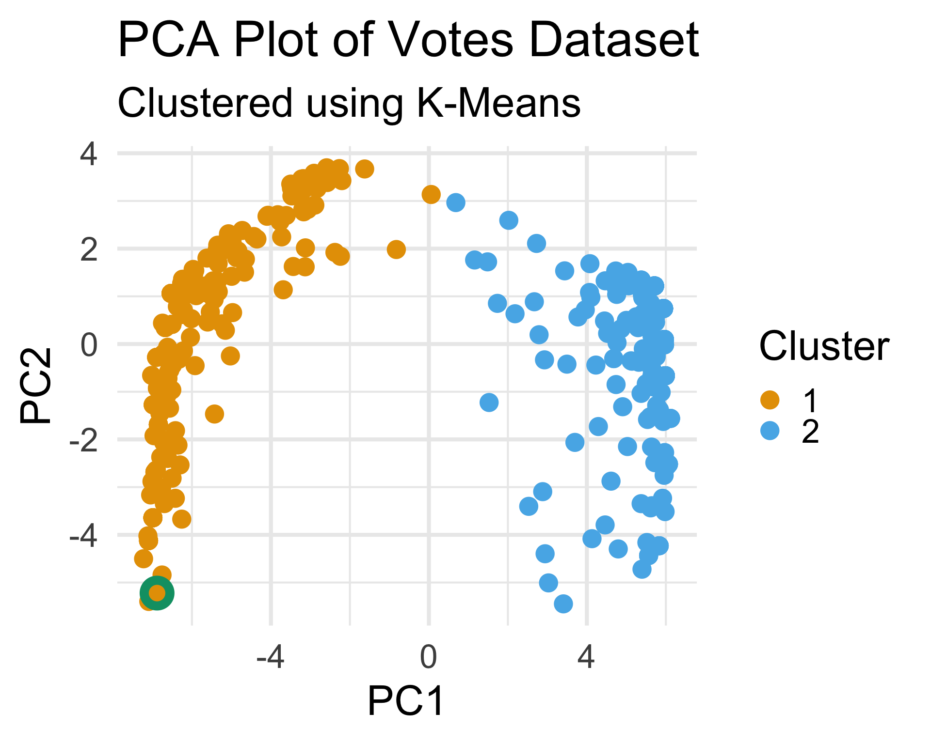
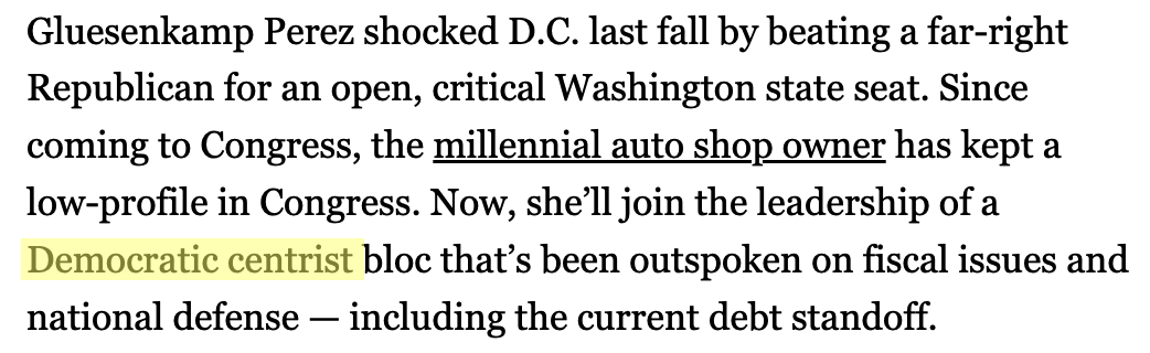
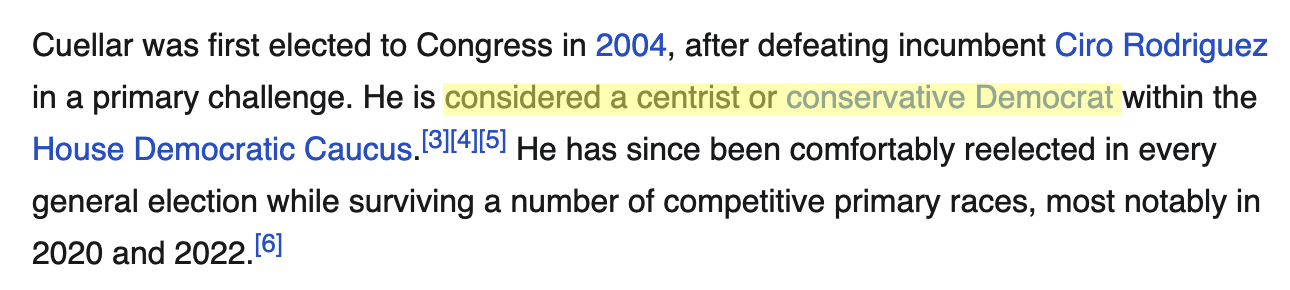
This person falls well within our “Democratcic” cluster, meaning they are likely a Democrat.
In this way, we can see that clustering can, in some cases, help us with missing data.
Indeed, perhaps this is a good segue into our next topic for today…