PSTAT 100: Lecture 16

Regression, Part III

Ethan P. Marzban

Department of Statistics and Applied Probability; UCSB

Summer Session A, 2025

\[ \newcommand\R{\mathbb{R}} \newcommand{\N}{\mathbb{N}} \newcommand{\E}{\mathbb{E}} \newcommand{\Prob}{\mathbb{P}} \newcommand{\F}{\mathcal{F}} \newcommand{\1}{1\!\!1} \newcommand{\comp}[1]{#1^{\complement}} \newcommand{\Var}{\mathrm{Var}} \newcommand{\SD}{\mathrm{SD}} \newcommand{\vect}[1]{\vec{\boldsymbol{#1}}} \newcommand{\tvect}[1]{\vec{\boldsymbol{#1}}^{\mathsf{T}}} \newcommand{\hvect}[1]{\widehat{\boldsymbol{#1}}} \newcommand{\mat}[1]{\mathbf{#1}} \newcommand{\tmat}[1]{\mathbf{#1}^{\mathsf{T}}} \newcommand{\Cov}{\mathrm{Cov}} \DeclareMathOperator*{\argmin}{\mathrm{arg} \ \min} \newcommand{\iid}{\stackrel{\mathrm{i.i.d.}}{\sim}} \]

Categorical Predictors

Mario Kart

• Let’s consider a dataset pertaining to Mario Kart.
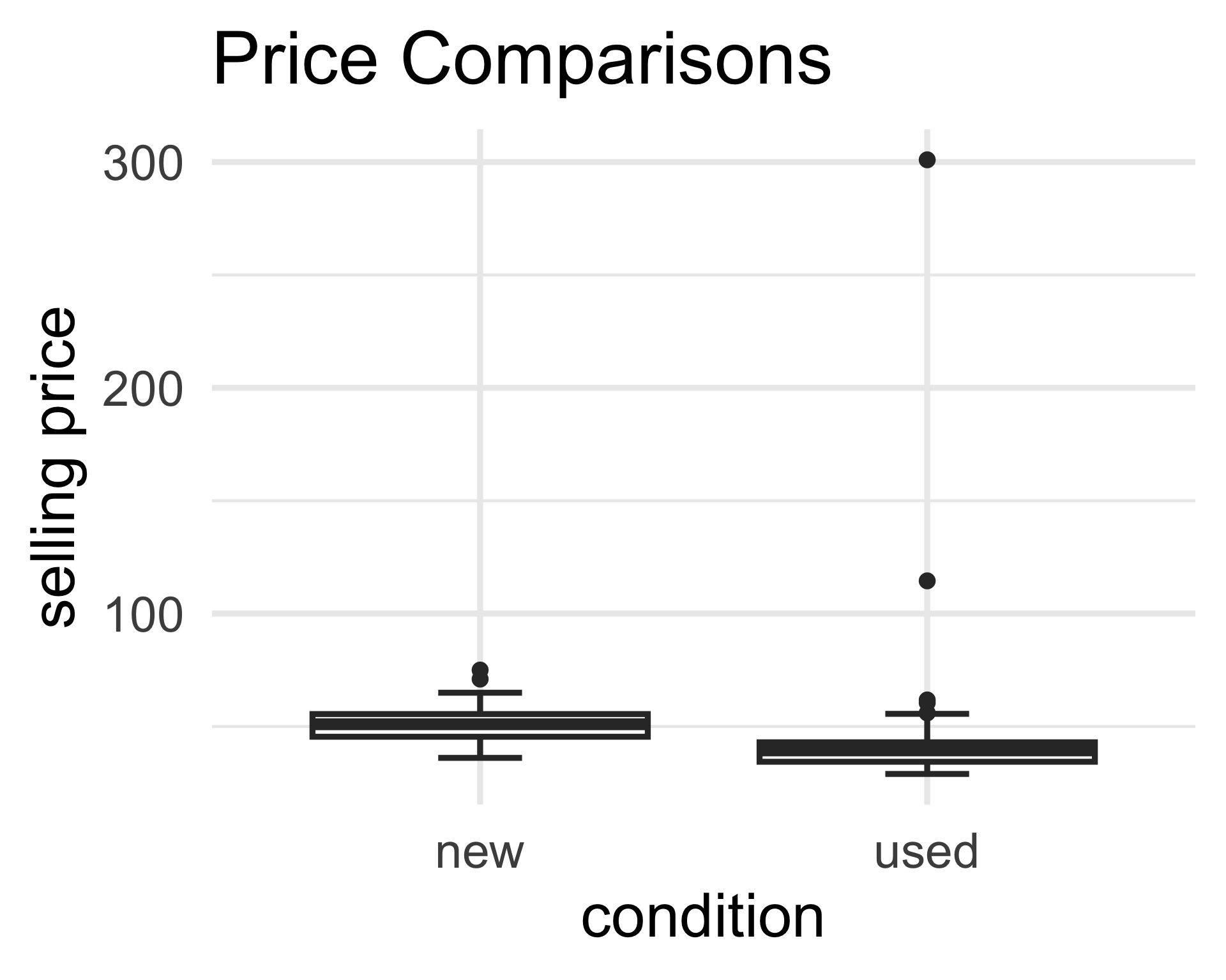
  • Specifically, this dataset tracks the selling price of used and new copies of Mario Kart for the Nintendo Wii.

sell_price	cond
47.55	new
33.05	used
42	new
44	new
71	new
41	new
37.02	used

Mario Kart

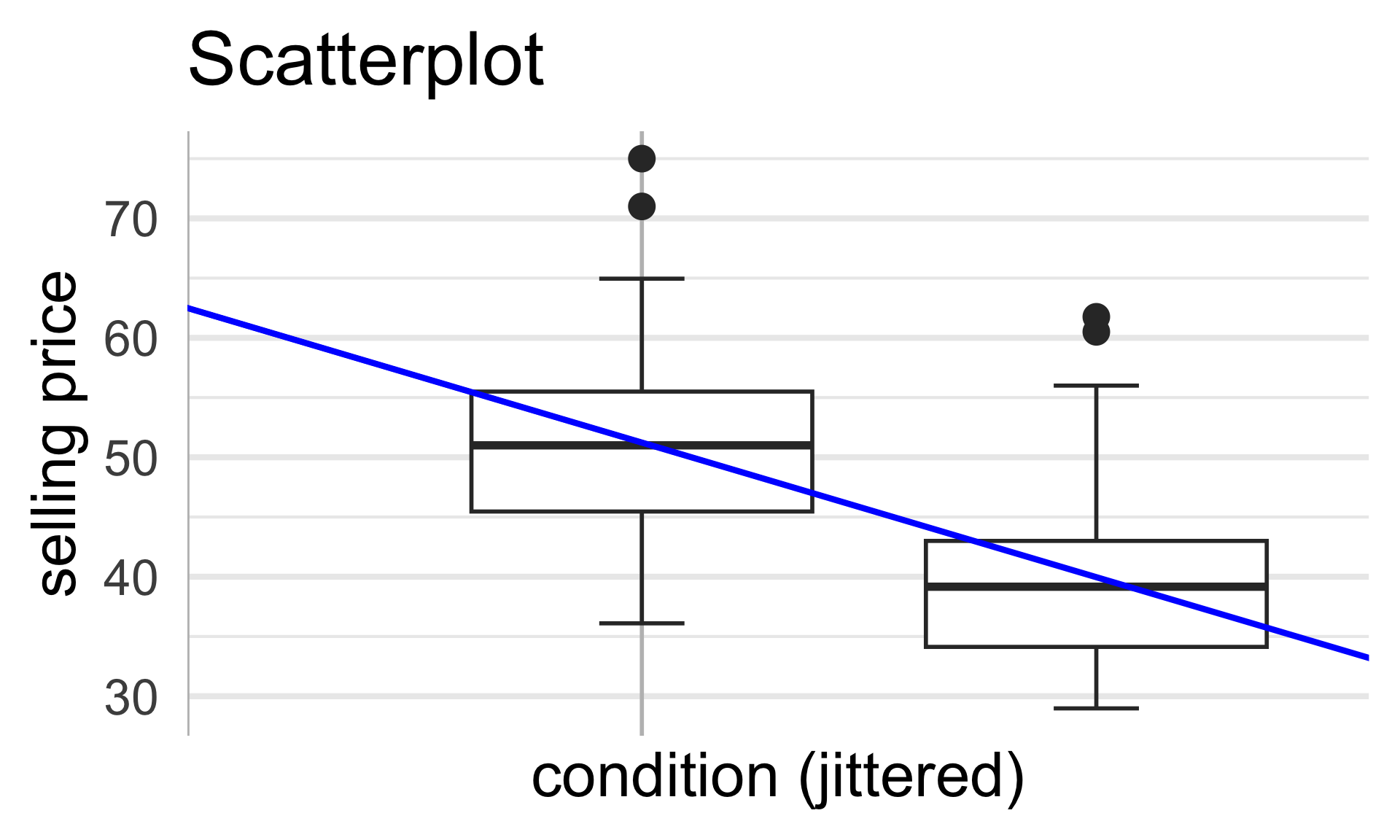
• Let’s remove the two unusually-expensive used copies from our consideration.
  • Very likely, these were rare/antique copies which is why they sold for unusually high prices

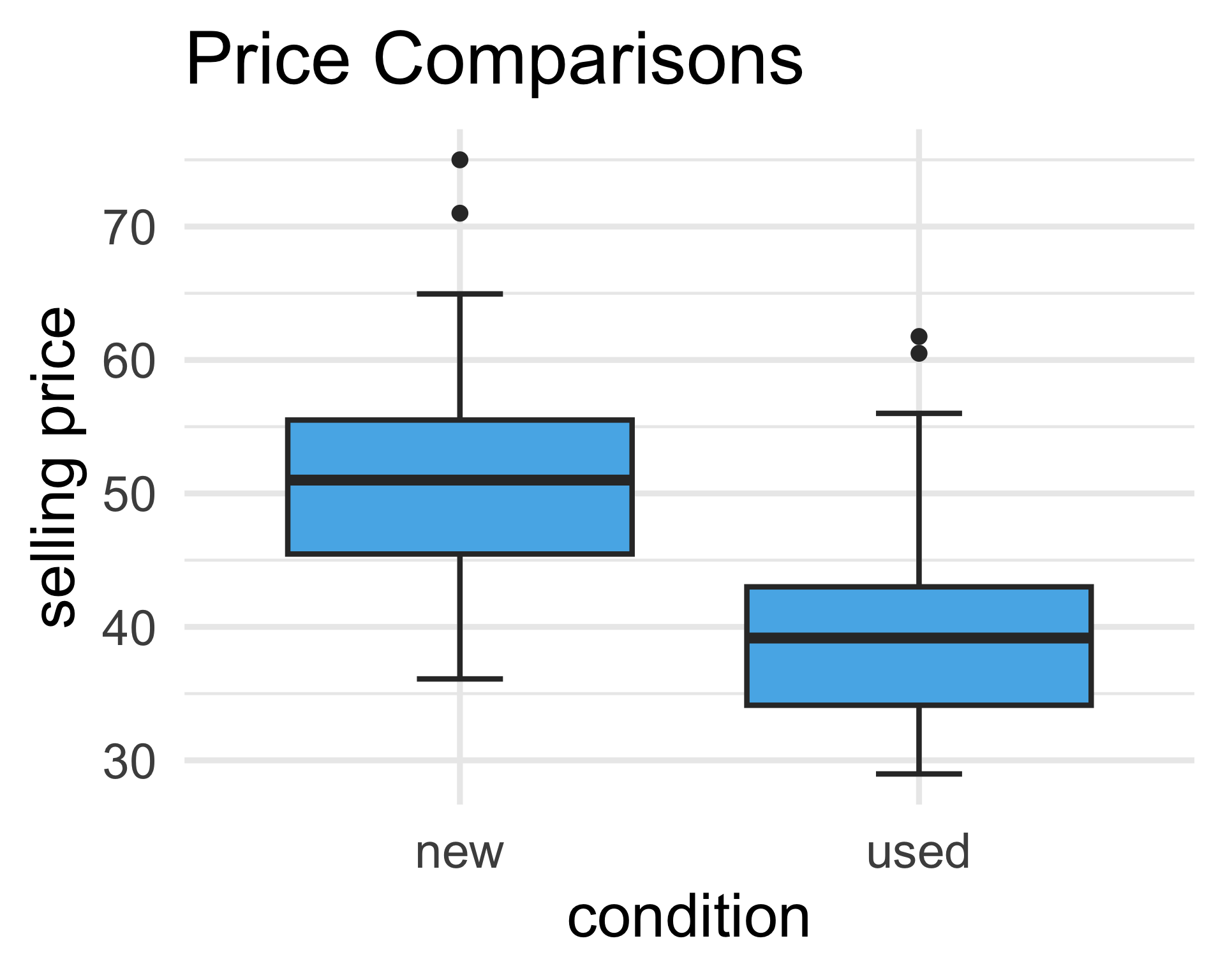
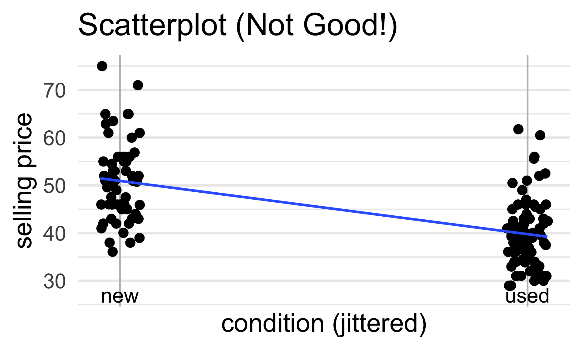
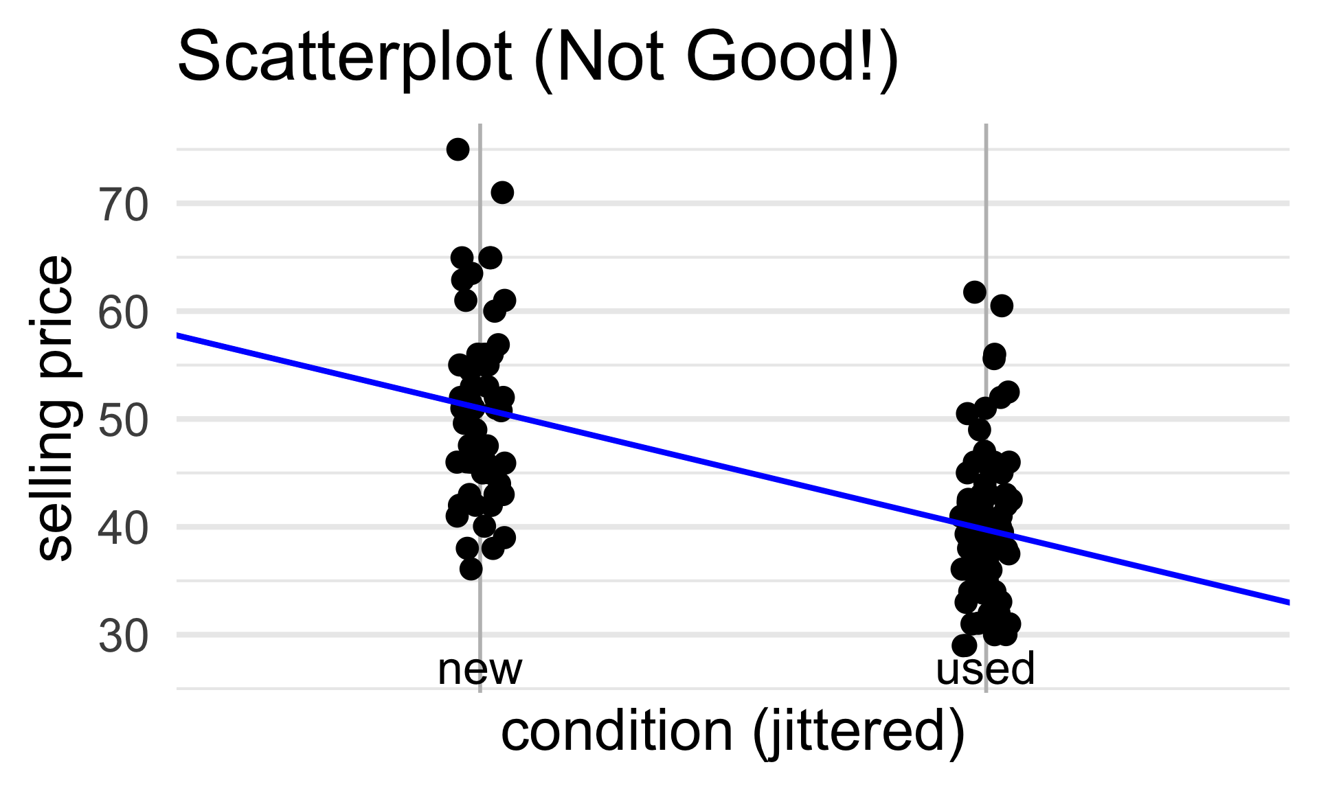
• From our plot, it appears as though, on average, used copies sold for less than new copies.

• But how might we model this statistically?

• y_i = β₀ + β₁ x_i + ε_i?

Mario Kart

sell_price	cond
47.55	new
33.05	used
42	new

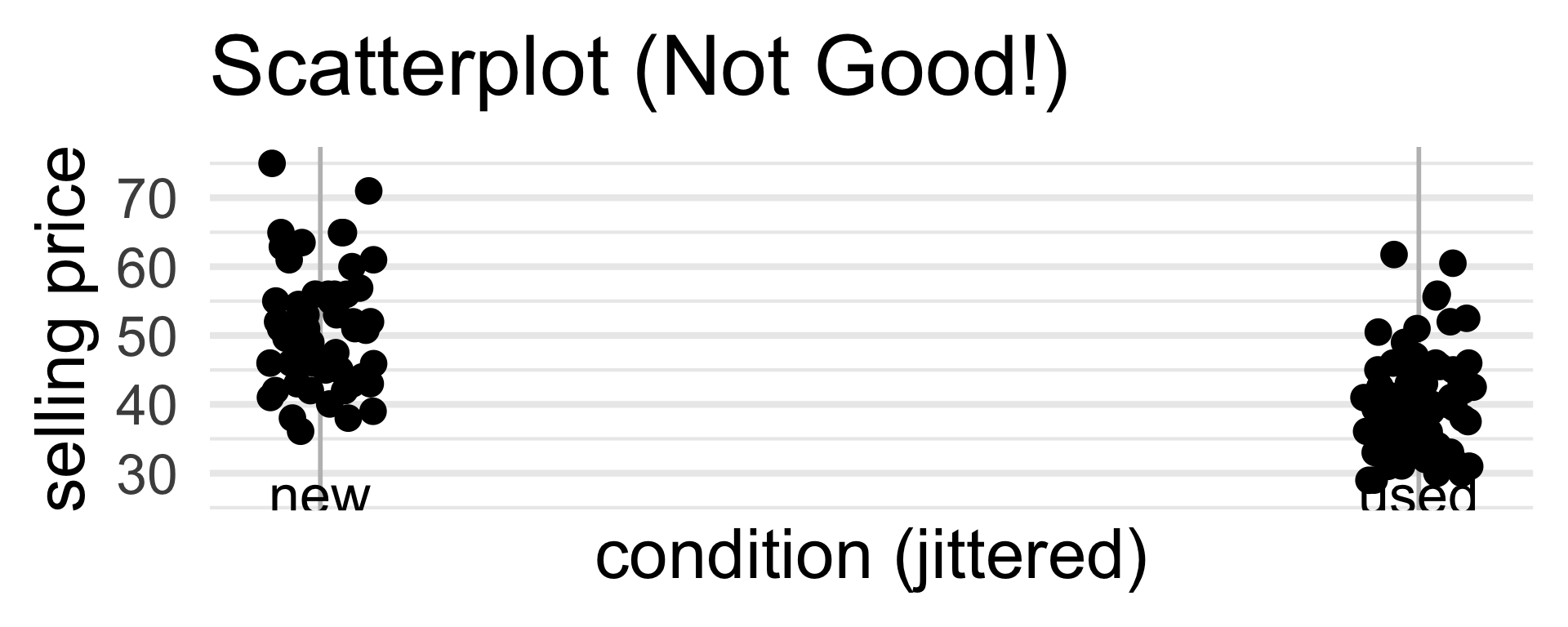
• By the way, recall that a “scatterplot” is NOT a good plot for this particular dataset - I’m mainly including one to keep things consistent with out treatment of regression from the past few lectures.

• 47.55 = β₀ + β₁ (new) + ε_i? That doesn’t seem right…

• The main idea is that our covariate is now categorical (as opposed to numerical). So, we need a new way to encode its observations into our model.

• Idea: use indicators!

Mario Kart

sell_price	cond
47.55	new
33.05	used
42	new

\[ y_i = \beta_0 + \beta_1 \cdot 1 \! \! 1 \{ \texttt{condition}_i = \texttt{used} \} + \varepsilon_i \]

Mario Kart

sell_price	cond
47.55	new
33.05	used
42	new

\[ y_i = \begin{cases} \beta_0 + \beta_1 + \varepsilon_i & \text{if $i^\text{th}$ copy is used} \\ \beta_0 + \varepsilon_i & \text{if $i^\text{th}$ copy is new} \\ \end{cases} \]

• β₀ can be interpreted as the average price among new copies
• β₀ + β₁ can be interpreted as the average price among used copies
  • Hence, β₁ can be interpreted as the average difference in price between new and used copies of the game

Mario Kart

\[ \widehat{y}_i = \beta_0 + \beta_1 1 \! \! 1\{\texttt{condition}_i = \texttt{used}\} \]

cond	avg_price
new	51.01
used	39.74

Coefficients:
            Estimate Std. Error t value Pr(>|t|)    
(Intercept)   51.008      0.995  51.266  < 2e-16 ***
condused     -11.271      1.305  -8.639  1.2e-14 ***

• Note: 39.74 - 51.0 = -11.26.

Mario Kart

• Before, we used the indicator \(1 \! \! 1 \{ \texttt{condition}_i = \texttt{used} \}\). What happens if we, instead, used the indicator \(1 \! \! 1 \{ \texttt{condition}_i = \texttt{new} \}\)?

• Mathematically, our model becomes

\[ y_i = \beta_0 + \beta_1 1 \! \! 1 \{ \texttt{condition}_i = \texttt{new} \} + \varepsilon_i = \begin{cases} \beta_0 + \beta_1 + \varepsilon_i & \text{if $i^\text{th}$ game is new} \\ \beta_0 + \varepsilon_i & \text{if $i^\text{th}$ game is used} \\ \end{cases} \]

• Now, β₀ can be interpreted as the average selling price among used copies and β₀ + β₁ can be interpreted as the average selling price among new copies.
  • Then, β₁ represents the difference in average selling prices between new and used copies.
• Question: What are the new estimates of the slope and intercept?

Encoding Binary Variables

0/1 Encoding

• In our previous example, our covariate (game condition) was categorical.
  • Specifically, it is what we might call binary, since its values are one of only two possibilities (used or new).
• In the case of a general binary covariate x, we need to select which level (i.e. category) corresponds to a 0 value in our indicator and which corresponds to a 1 value in our indicator.
  • The level encoded with a 0 value is called the baseline (aka reference) level.
  • The intercept in an SLR will correspond to the average response value within the baseline level.
• It is up to you to set the baseline level; as we saw in Mario Kart example, our choice doesn’t matter too much as long as we are consistent!

Encoding Binary Variables

0/1 Encoding

• In R, the baseline level is set to whichever level of the factor appears first:

mariokart$cond %>% levels()

[1] "new"  "used"

• Since "new" appears as the first level, it was assigned to be the baseline level.

• If we want to recode the baseline, we can use the relevel() function:

mariokart <- mariokart %>% 
  mutate(cond_2 = relevel(cond, "used"))

mariokart$cond_2 %>% levels()

[1] "used" "new" 

Encoding Binary Variables

-1/1 Encoding

• The framework above is sometimes called 0/1 encoding, as we are using indicators (which output either a 0 or a 1 value).

• There is another type of encoding commonly used, called -1/1 encoding.

• As the name suggests, instead of assigning 0/1 values to the categories, we assign -1/1 values.

• For example, in the Mario Kart example, we might set \[ x_i = \begin{cases} +1 & \text{if the $i^\text{th}$ copy was used} \\ -1 & \text{if the $i^\text{th}$ copy was new} \\ \end{cases} \]

Encoding Binary Variables

-1/1 Encoding

• Then, our model becomes

\[ y_i = \beta_0 + \beta_1 x_i + \varepsilon_i = \begin{cases} \beta_0 + \beta_1 + \varepsilon_i & \text{if $i^\text{th}$ game is used} \\ \beta_0 - \beta_1 - \varepsilon_i & \text{if $i^\text{th}$ game is used} \\ \end{cases} \]

• β₀ can be interpreted as the overall average price of game copies (ignoring condition entirely) β₁ can be interpreted as the amount over the average that new copies sell for and also the amount under the average that used copies sell for.

Encoding Binary Variables

-1/1 Encoding

mariokart$cond_2 <- ifelse(mariokart$cond == "new", 1, -1)
lm(sell_price ~ cond_2, mariokart) %>% summary()

Call:
lm(formula = sell_price ~ cond_2, data = mariokart)

Residuals:
     Min       1Q   Median       3Q      Max 
-14.9078  -5.7366  -0.2266   3.9822  23.9922 

Coefficients:
            Estimate Std. Error t value Pr(>|t|)    
(Intercept)  45.3722     0.6523  69.552  < 2e-16 ***
cond_2        5.6356     0.6523   8.639  1.2e-14 ***
---
Signif. codes:  0 '***' 0.001 '**' 0.01 '*' 0.05 '.' 0.1 ' ' 1

Residual standard error: 7.642 on 139 degrees of freedom
Multiple R-squared:  0.3493,    Adjusted R-squared:  0.3447 
F-statistic: 74.63 on 1 and 139 DF,  p-value: 1.203e-14

Encoding Binary Variables

-1/1 Encoding

mariokart %>% group_by(cond) %>% summarise(avg_price = mean(sell_price)) %>% pander()

cond	avg_price
new	51.01
used	39.74

(mariokart %>% 
    group_by(cond) %>% 
    summarise(avg_price = mean(sell_price))
)$avg_price %>% mean()

[1] 45.37219

Encoding Categorical Variables

Multiple Levels

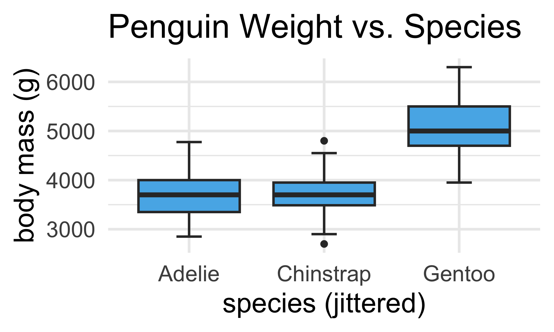
• What if we have a covariate with more than two levels?

• As an example, let’s return to the palmerpenguins dataset

  • Recall that this particular dataset tracks various characteristics of penguins from the Palmer Research Station in Antarctica

• One variable records the species of each penguin, as either Adélie, Chinstrap, or Gentoo
  • As such, species is a categorical variable that has three levels.

Artwork by @allison_horst

Encoding Categorical Variables

Palmerpenguins species

body_mass_g	species
3750	Adelie
3800	Adelie
3250	Adelie
NA	Adelie
3450	Adelie

\[\begin{align*} y_i & = \beta_0 + \beta_1 1 \! \! 1 \{\texttt{species}_i = \texttt{Adelie}\} + \beta_2 1 \! \! 1 \{\texttt{species}_i = \texttt{Chinstrap}\} \\ & \hspace{15mm} + \beta_3 1 \! \! 1 \{\texttt{species}_i = \texttt{Gentoo}\} + \varepsilon_i \end{align*}\]

• What’s the intercept β₀ doing here? (Hint: how many species are there?)

Encoding Categorical Variables

Palmerpenguins species

\[\begin{align*} y_i & = \beta_0 + \beta_1 1 \! \! 1 \{\texttt{species}_i = \texttt{Chinstrap}\} \\ & \hspace{15mm} + \beta_2 1 \! \! 1 \{\texttt{species}_i = \texttt{Gentoo}\} + \varepsilon_i \end{align*}\]

• Here, we’ve set Adelie to be the baseline level.
  • Said differently, β₀ can now be interpreted as the average body weight of Adélie penguins.
• The slope parameters can now be interpreted as comparisons of species-specific body weights as compared to the average body weight of Adélie penguins.
  • E.g. β₁ represents the average difference in body weights of Chinstrap penguins as compared with Adélie penguins.

Encoding Categorical Variables

General Case

• In general, for a categorical variable with k levels, we will (if we want to use proper indicators to encode values) need only k – 1 slope parameters and one intercept (representing the average response value within the baseline level).

• This is often called a set-to-zero condition, as we are explicitly setting one of the parameters (i.e. one of the slope parameters) to be equal to zero.

• There exists another type of condition, which we will not discuss in this course (but will arise in future classes, like PSTAT 122).

Your Turn!

Your Turn!

Interpret the following R output:

Call:
lm(formula = body_mass_g ~ species, data = penguins)

Residuals:
     Min       1Q   Median       3Q      Max 
-1126.02  -333.09   -33.09   316.91  1223.98 

Coefficients:
                 Estimate Std. Error t value Pr(>|t|)    
(Intercept)       3700.66      37.62   98.37   <2e-16 ***
speciesChinstrap    32.43      67.51    0.48    0.631    
speciesGentoo     1375.35      56.15   24.50   <2e-16 ***
---
Signif. codes:  0 '***' 0.001 '**' 0.01 '*' 0.05 '.' 0.1 ' ' 1

Residual standard error: 462.3 on 339 degrees of freedom
  (2 observations deleted due to missingness)
Multiple R-squared:  0.6697,    Adjusted R-squared:  0.6677 
F-statistic: 343.6 on 2 and 339 DF,  p-value: < 2.2e-16

03:00

An Interesting Connection…

sell_price	cond
47.55	new
33.05	used
42	new
44	new
71	new

\[ y_i = \beta_0 + \beta_1 \cdot 1 \! \! 1 \{ \texttt{condition}_i = \texttt{used} \} + \varepsilon_i \]

An Interesting Connection…

sell_price	cond
47.55	new
33.05	used
42	new
44	new
71	new

\[ y_i = \beta_0 + \beta_1 \cdot 1 \! \! 1 \{ \texttt{condition}_i = \texttt{used} \} + \varepsilon_i \]

An Interesting Connection…

sell_price	cond
47.55	new
33.05	used
42	new
44	new
71	new

y = (grand mean) + (deviations from grand mean) + (noise)

This is just ANOVA!

\[ y_{ij} = \mu + \tau_j + \varepsilon_{ij}; \quad i = 1, \cdots, n_j; \ j = 1, 2 \]

An Interesting Connection…

aov(mariokart$sell_price ~ mariokart$cond) %>% coef()

       (Intercept) mariokart$condused 
          51.00780          -11.27121 

lm(mariokart$sell_price ~ mariokart$cond) %>% coef()

       (Intercept) mariokart$condused 
          51.00780          -11.27121 

Moral

Regression with categorical variables is equivalent to ANOVA.

ANOVA Tables

• This also allows us to address one oustanding issue: that of the output of aov().

• Back when we talked about ANOVA, I mentioned we’d discuss the output of aov() a bit more after we discussed regression.

• This is because an ANOVA Table is really just a regression table!

aov(mariokart$sell_price ~ mariokart$cond) %>% summary()

                Df Sum Sq Mean Sq F value  Pr(>F)    
mariokart$cond   1   4359    4359   74.63 1.2e-14 ***
Residuals      139   8119      58                    
---
Signif. codes:  0 '***' 0.001 '**' 0.01 '*' 0.05 '.' 0.1 ' ' 1

Your Turn!

Your Turn!

Using the penguins dataset, regress body mass onto flipper length, flipper depth, species, and sex.

1. Should any covariates be removed from the model? Why?
2. Produce a regression table and interpret the results. (If you believe a covariate should be removed, produce a regression table for the modified regression fit, after removing the covariate.)

06:00

An Important Distinction

• Note that our discussions today have all been about categorical covariates.

• We have still been in a regression setting; i.e. assuming that our response is numerical.

• The question of how to deal with categorical responses leads us into the realm of classification, which we will start discussing tomorrow.

• For now, I’d like to close our our Regression chapter with some extensions.

Series Estimators

Recap

Statistical Model

y = f ( x ) + noise

• As mentioned a few lectures ago, in parametric modeling, we decompose the signal into a series of components, each involving a parameter that can be estimated.

• For instance, in linear regression, we asserted yi = β₀ + β₁ x_i,1 + … + β_p x_i,p + ε_i

  • Estimating the signal is therefore equivalent to estimating the parameters.

• There exist other approaches to regression, some of which we will briefly discuss now.

Polynomial Regression

• Recall polynomial regression: yi = β₀ + β₁ xi + β₂ xi² + … + β_p xi^p + ε_i

• Polynomial regression is actually a special case of a broader class of regression techniques, called series estimators (sometimes called basis regression methods).

• The idea is that we continue to decompose our signal function into a series of estimable components; now, however, we use a set of orthonormal basis function \(\{\phi_k(t)\}_{k}\): \[ f(x) = \sum_{k = 0}^{p} \beta_k \phi_k(x) \]

Polynomial Regression

• For example, polynomial regression essentially takes \(\phi_k(x) = x^k\)
  • Aside: “raw” polynomials (x, x², etc.) are not orthogonal, so technically we use an orthogonalized version of polynomials (e.g. Legendre polynomials or Hermite polynomials).

Piecewise Regression

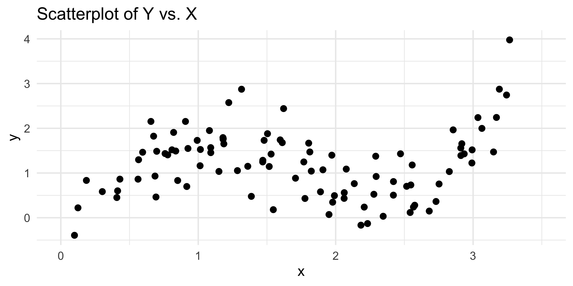
Example Data

Piecewise Regression

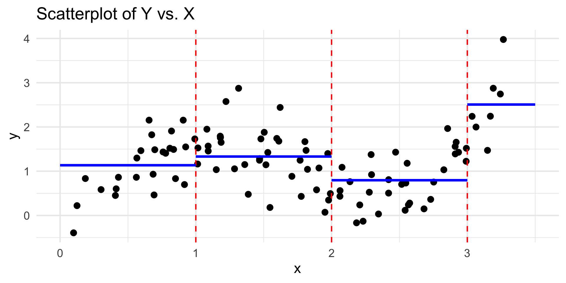
Piecewise-Constant Regression

Piecewise Regression

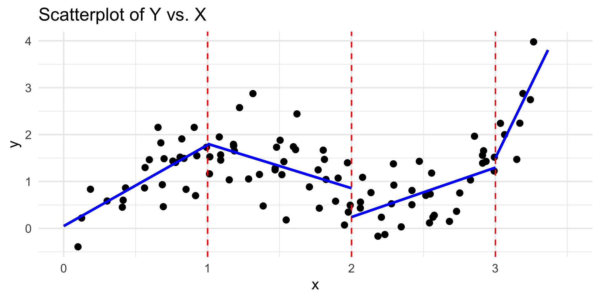
Piecewise-Linear Regression

Piecewise Regression

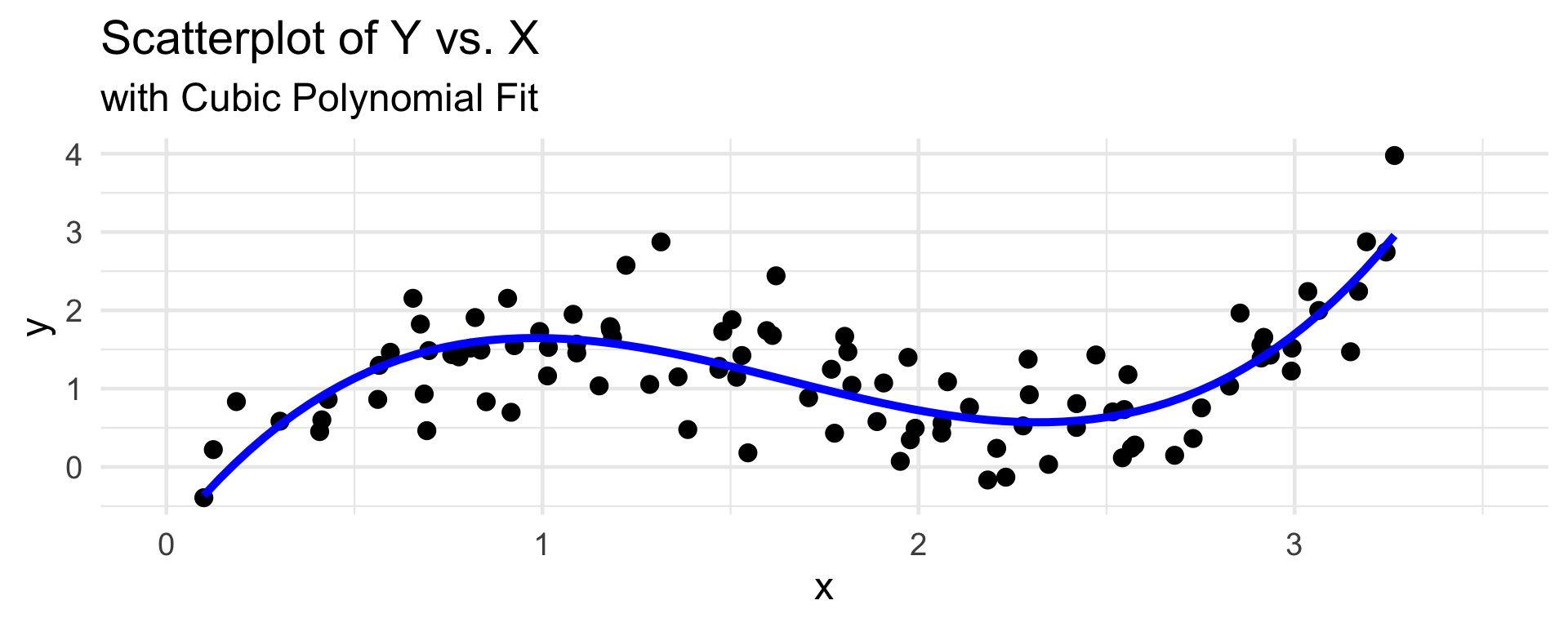
Piecewise-Cubic Regression

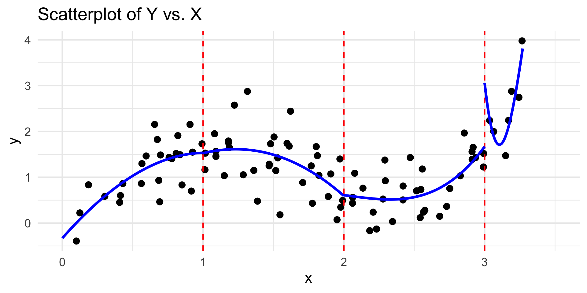
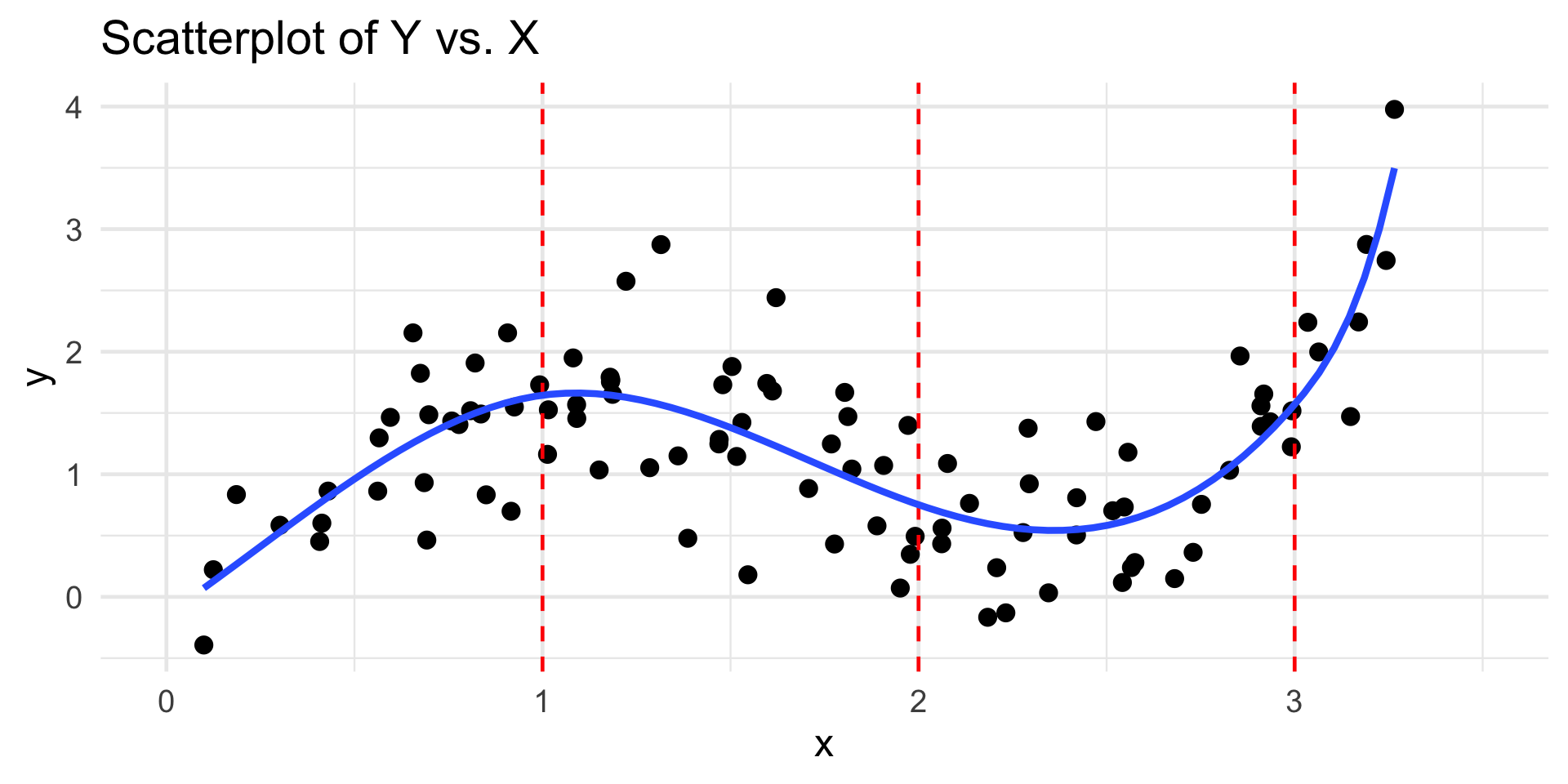
Piecewise Regression

Piecewise-Cubic Regression with Boundary Conditions

Piecewise Regression

Splines

• Piecewise-polynomial regression is actually also an example of a series estimator!
  • Essentially we take \(\phi_k(x) = x^k \cdot 1 \! \! 1_{\{c_k \leq x < c_{k + 1}\}}\)
• Piecewise-cubic regression with the constraint of being continuous and twice-differentiable at the endpoints is called spline regression. The points at which we divide our data are called knots.
  • Again, we won’t cover how to select the location or number of knots; you’ll talk more about this in PSTAT 131/231.

Series Estimators

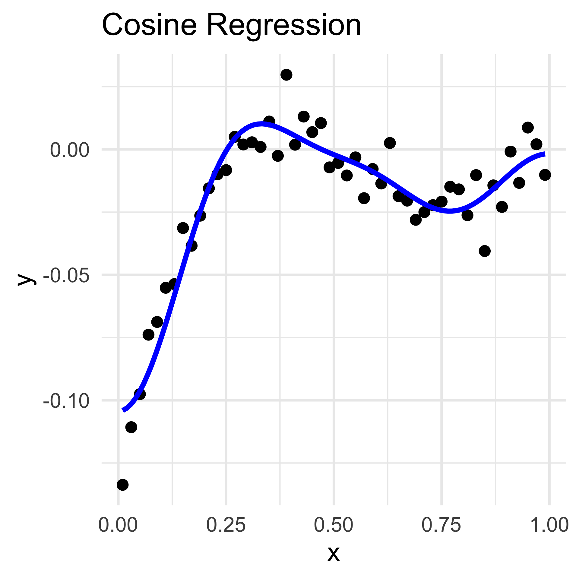
Trigonometric Regression

• Assuming equally-spaced inputs, we can also propose a class of trigonometric series estimators; for example,

\[ f(x) = \sum_{j=1}^{p} \beta_j \cos[(j - 1) \pi x]\]

• Selection of p can be accomplished with Cross-Validation (out-of-scope for PSTAT 100)

Series Estimators

Kernel Regression

• Inspired by our discussion on Kernel Density Estimation, we can propose a kernel regression estimate:

\[ \widehat{f}(x) = \frac{1}{n \lambda} \sum_{i=1}^{n}\left[ K\left(\frac{x - x_i}{\lambda} \right)y_i \right] \]

• Estimators like these arise frequently in a class like PSTAT 105, and are widely categorized as a nonparametric regression technique.
  • Fun Fact: my own research falls within the paradigm of nonparametric regression!
  • Essentially, my advisor and I are trying to propose a new nonparametric regression estimator that allows for correlation in the outputs.

Next Time

• Tomorrow we’ll begin (and conclude) our discussion on Classification.

• Lab 08 (tomorrow’s lab) will walk you through some hands-on explorations of classification.

  • As a reminder, if you attend Section in-person tomorrow you will gain access to the solutions to Lab 08 early!

• I advise you to keep working through the ICA 02 practice problems as well.