PSTAT 100: Lecture 14

Simple Linear Regression

Ethan P. Marzban

Department of Statistics and Applied Probability; UCSB

Summer Session A, 2025

\[ \newcommand\R{\mathbb{R}} \newcommand{\N}{\mathbb{N}} \newcommand{\E}{\mathbb{E}} \newcommand{\Prob}{\mathbb{P}} \newcommand{\F}{\mathcal{F}} \newcommand{\1}{1\!\!1} \newcommand{\comp}[1]{#1^{\complement}} \newcommand{\Var}{\mathrm{Var}} \newcommand{\SD}{\mathrm{SD}} \newcommand{\vect}[1]{\vec{\boldsymbol{#1}}} \newcommand{\Cov}{\mathrm{Cov}} \DeclareMathOperator*{\argmin}{\mathrm{arg} \ \min} \newcommand{\iid}{\stackrel{\mathrm{i.i.d.}}{\sim}} \]

Recap

Statistical Modeling

Yesterday, we discussed the general framework of statistical models.
- We discussed this in the context of one random variable (e.g. modeling flips of a coin), and two variables (regression and classification).
Given a response y and an explanatory variable x, the most general form for a model is y = f ( x ) + noise
- For instance, we explored how the median selling price of a house in 2014 can be modeled as a function of the year in which it was built.
Regression models arise when the response is numerical; classification models arise when the response is categorical.

Recap

Types of Statistical Models

Check Your Understanding

Identify the following situations as either regression or classification:

Predicting the birth weight of a newborn from the mothers’ height, blood type, and white blood cell count
Predicting whether or not a newborn will be born with a congenital heart defect or not, based on the mother and fathers’ health history.
Describing the relationship between the number of accidents on a stretch of highway and: the number of cars driving, the speed limit, and the time of day.

Penguins

An Example

The penguins dataset, from the palmerpenguins package, contains information on 344 penguins, collected by Dr. Kristen Gorman, at the Palmer Research Station in Antarctica.
Three species of penguins were observed: Adélie, Chinstrap, and Gentoo

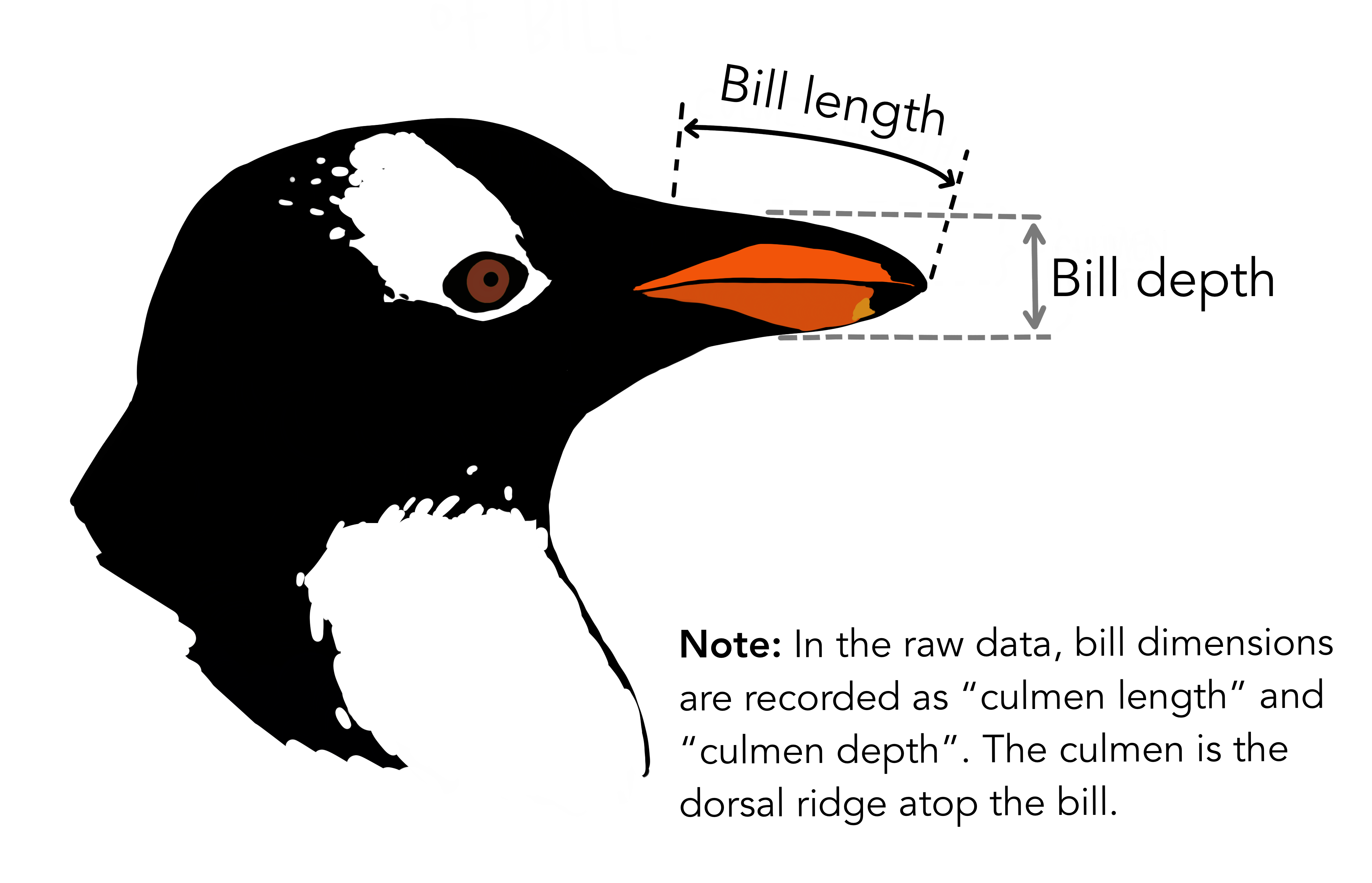
Various characteristics of each penguin were also observed, including: flipper length, bill length, bill depth, sex, and island.
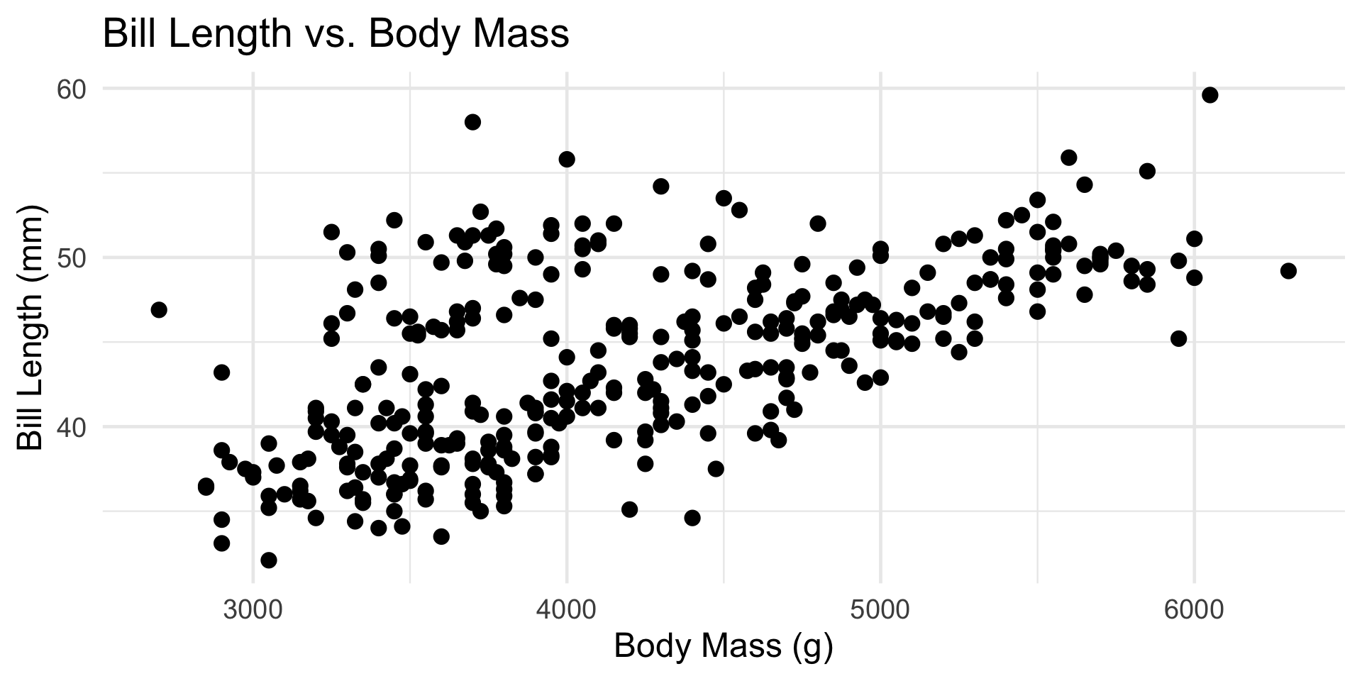
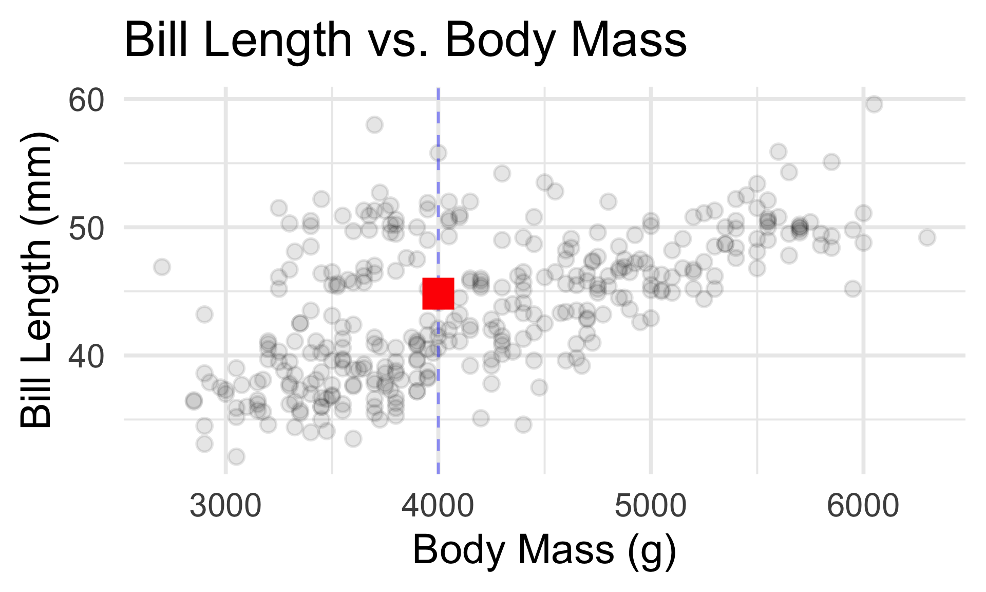
It seems plausible that a penguin’s bill length should be related to its body mass.

Penguins

An Example

Code

penguins %>% ggplot(aes(x = body_mass_g, y = bill_length_mm)) +
  geom_point(size = 3) + 
  theme_minimal(base_size = 18) + 
  xlab("Body Mass (g)") + ylab("Bill Length (mm)") +
  ggtitle("Bill Length vs. Body Mass")

Based on our discussions from Week 1:
- Is there a trend?
- Increasing or decreasing?
- Linear or nonlinear?

If we model Bill Length (response) as a function of Body Mass (predictor), would this be a regression or a classification model?

Penguins

Step 1: Propose a Model

y_i = β₀ + β₁ x_i + ε_i

y_i = i^th Bill Length measurement
x_i = i^th Body Mass measurement
ε_i = i^th (aleatoric) noise term
- We simply assume, for now, that the noise is mean zero (𝔼[ε_i] = 0 for all i) and homoskedastic (constant variance; Var(ε_i) = σ², across all i)

Simple Linear Regression Model

Step 1: Propose a Model

y_i = β₀ + β₁ x_i + ε_i

y_i = i^th response measurement
x_i = i^th predictor measurement
ε_i = i^th (aleatoric) noise term; zero-mean and homoskedastic

Called the Simple Linear Regression (SLR) model.
- Simple: only one covariate
- Linear: we are assuming a linear signal function
- Regression: well, you tell me!

Simple Linear Regression Model

As Applied to the `Palmerpenguins` Dataset

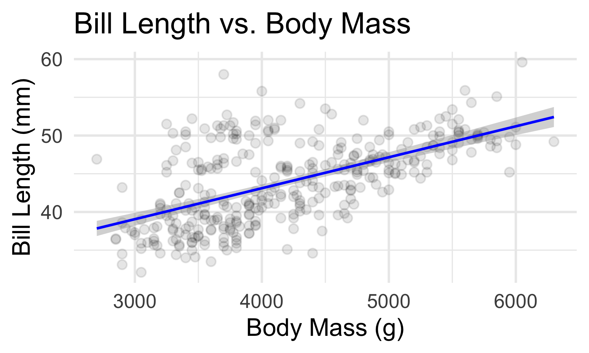
Essentially, the SLR seeks to fit the “best” line to the data.
The parameters that need to be estimated in the model fitting step are, therefore, the intercept and the slope.

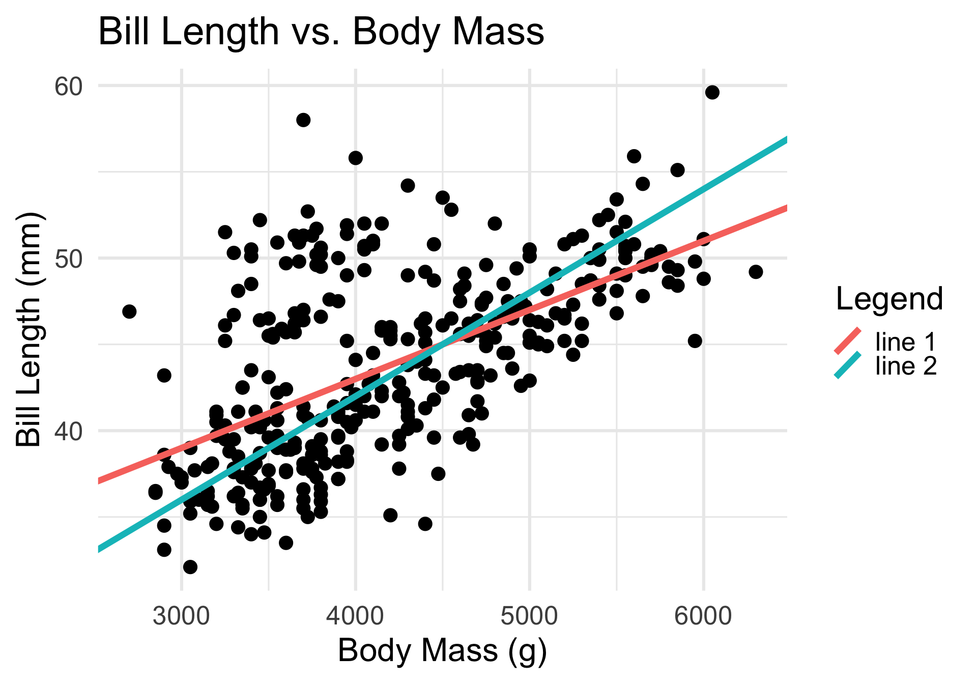
Identifying these slope and intercept values by eye is next to impossible - this is why modeling is so useful!

Simple Linear Regression Model

Step 2: Fit the Model to the Data

Let’s find the optimal slope and intercept using the “loss” framework introduced in lecture yesterday.
Specifically, for each y_i we believe there to be a “true response” value given by β₀ + β₁ x_i, where β₀ and β₁ are the true slope and intercept.
- Given estimates b₀ and b₁ for β₀ and β₁, respectively, our “best guess” at this true response value is simply b₀ + b₁ x_i.
So, adopting L₂ loss, let’s take \(\mathcal{L}(y_i, b_0, b_1) := (y_i - b_0 - b_1 x_i)^2\) so that our empirical risk becomes

\[ R(b_0, b_1) = \frac{1}{n} \sum_{i=1}^{n} (y_i - b_0 - b_1 x_i)^2 \]

Simple Linear Regression Model

Step 2: Fit the Model to the Data

Our “best” estimators are then those b₀ and b₁ values that minimize this above quantity.
- Such ideal estimators - namely, those that minimize empirical risk under squared loss - are called the ordinary least-squares (OLS) estimators/estimates in the context of SLR.

\[ \begin{pmatrix} \widehat{\beta}_{0, \ \mathrm{OLS}} \\ \widehat{\beta}_{1, \ \mathrm{OLS}} \end{pmatrix} := \argmin_{(b_0, b_1)} \left\{ \frac{1}{n} \sum_{i=1}^{n} (y_i - b_0 - b_1 x_i)^2 \right\} \]

This is a simultaneous minimization problem in two dimensions, so we’ll need to take partial derivatives.

Simple Linear Regression

Step 2: Estimate Parameters

\[ R(b_0, b_1) = \frac{1}{n} \sum_{i=1}^{n} (y_i - b_0 - b_1 x_i)^2 \]

\[\begin{align*} \frac{\partial R}{\partial b_0} & = - \frac{2}{n} \sum_{i=1}^{n} (y_i - b_0 - b_1 x_i) \\ & = - \frac{2}{n} \left( n \overline{y}_n - n b_1 - n \overline{x}_n b_1 \right) \\ & = - 2 \left( \overline{y}_n - b_0 - \overline{x}_n b_1 \right) \end{align*}\]

\[\begin{align*} \frac{\partial R}{\partial b_1} & = - \frac{2}{n} \sum_{i=1}^{n} x_i (y_i - b_0 - b_1 x_i) \\ & = - \frac{2}{n} \left( n \overline{x}_n \overline{y}_n - n \overline{x}_n b_0 - b_1 \sum_{i=1}^{n} x_i^2 \right) \\ & = - 2 \left( \overline{x}_n \overline{y}_n - \overline{x}_n b_0 - \frac{1}{n} b_1 \sum_{i=1}^{n} x_i^2 \right) \end{align*}\]

Simple Linear Regression

Step 2: Estimate Parameters

\[\begin{align*} \overline{y}_n - \widehat{\beta}_0 - \overline{x}_n \widehat{\beta}_1 & = 0 \\ \overline{x}_n \overline{y}_n - \overline{x}_n \widehat{\beta}_0 - {\textstyle \frac{1}{n} \widehat{\beta}_1 \sum_{i=1}^{n} x_i^2 } & = 0 \end{align*}\]

We call these the normal equations. When solved, they reveal:

\[ \widehat{\beta}_0 = \overline{y}_n - \widehat{\beta}_1 \overline{x}_n; \qquad \widehat{\beta}_1 = r \cdot \frac{s_Y}{s_X} \] where s_X and s_Y denote the sample variances of the x and y values, respectively, and \[ r := \frac{1}{n - 1} \sum_{i=1}^{n} \left( \frac{x_i - \overline{x}_n}{s_X} \right) \left( \frac{y_i - \overline{y}_n}{s_Y} \right) \] denotes Pearson’s Correlation Coefficient.

Simple Linear Regression

set.seed(100)   ## for reproducibility
x <- rnorm(100)
y <- 0.5 + 1.5 * x + rnorm(100)

n <- length(x)
1/(n - 1) * sum(((x - mean(x))/sd(x)) * ((y - mean(y))/sd(y)))

[1] 0.8746656

cor(x, y)

[1] 0.8746656

beta1_hat <- cor(x, y) * sd(y) / sd(x)
beta0_hat <- mean(y) - beta1_hat * mean(x) 

cat("By Hand:", c(beta0_hat, beta1_hat), "\n",
    "From lm():", lm(y ~ x) %>% coef()
)

By Hand: 0.5114477 1.394633 
 From lm(): 0.5114477 1.394633

The function lm() - which stands for linear model - performs the model fitting step (under L₂ loss) for us.

Penguins

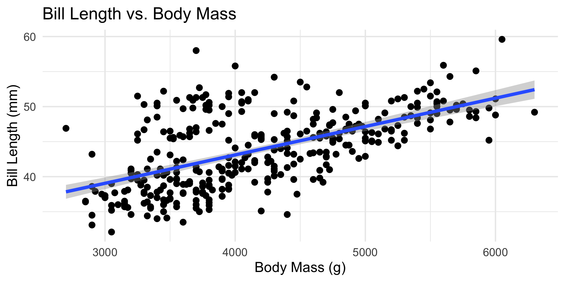
The Fitted SLR Model

Code

penguins %>% ggplot(aes(x = body_mass_g, y = bill_length_mm)) +
  geom_point(size = 3) + 
  theme_minimal(base_size = 18) + 
  xlab("Body Mass (g)") + ylab("Bill Length (mm)") +
  ggtitle("Bill Length vs. Body Mass") +
  geom_smooth(method = "lm", formula = y ~ x, linewidth = 2)

Model Diagnostics

Finally, let’s talk a bit about the third step in the modeling process: assessing model fit (sometimes called performing model diagnostics).
- Personally, I believe this is perhaps the most important step in the entire process!
Recall that the main goal of model diagnostics is to assess whether we believe our initial model (from step 1) is doing any good.
- To stress: even though, in step 2, we “optimized” our model, we are only optimizing under the model we picked. This says nothing about whether our choice of model was any good!

Model Diagnostics

Example: Poor Choice of Model

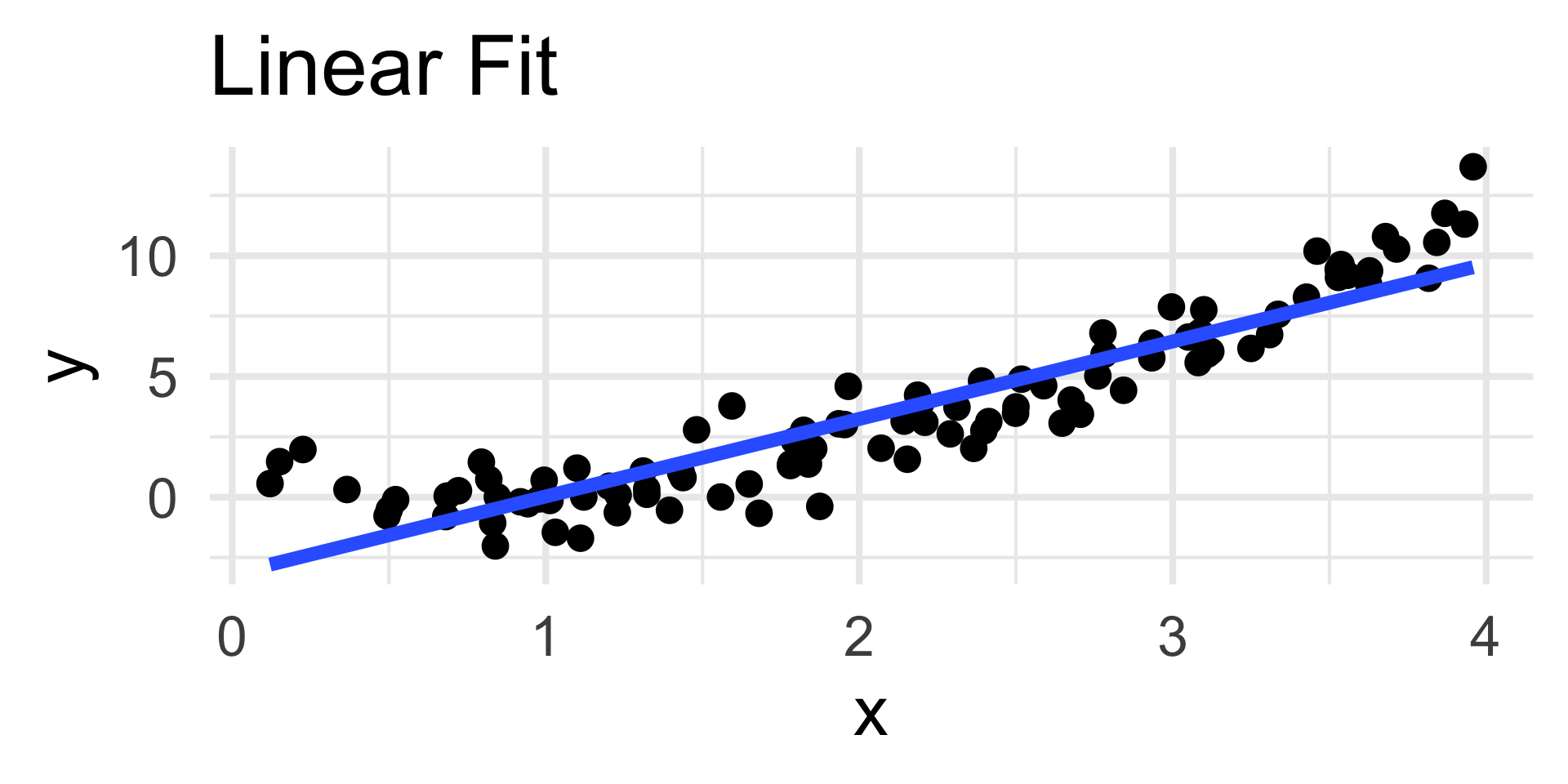
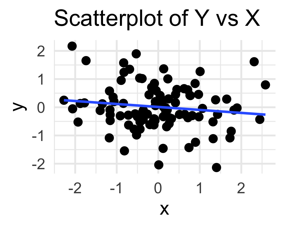
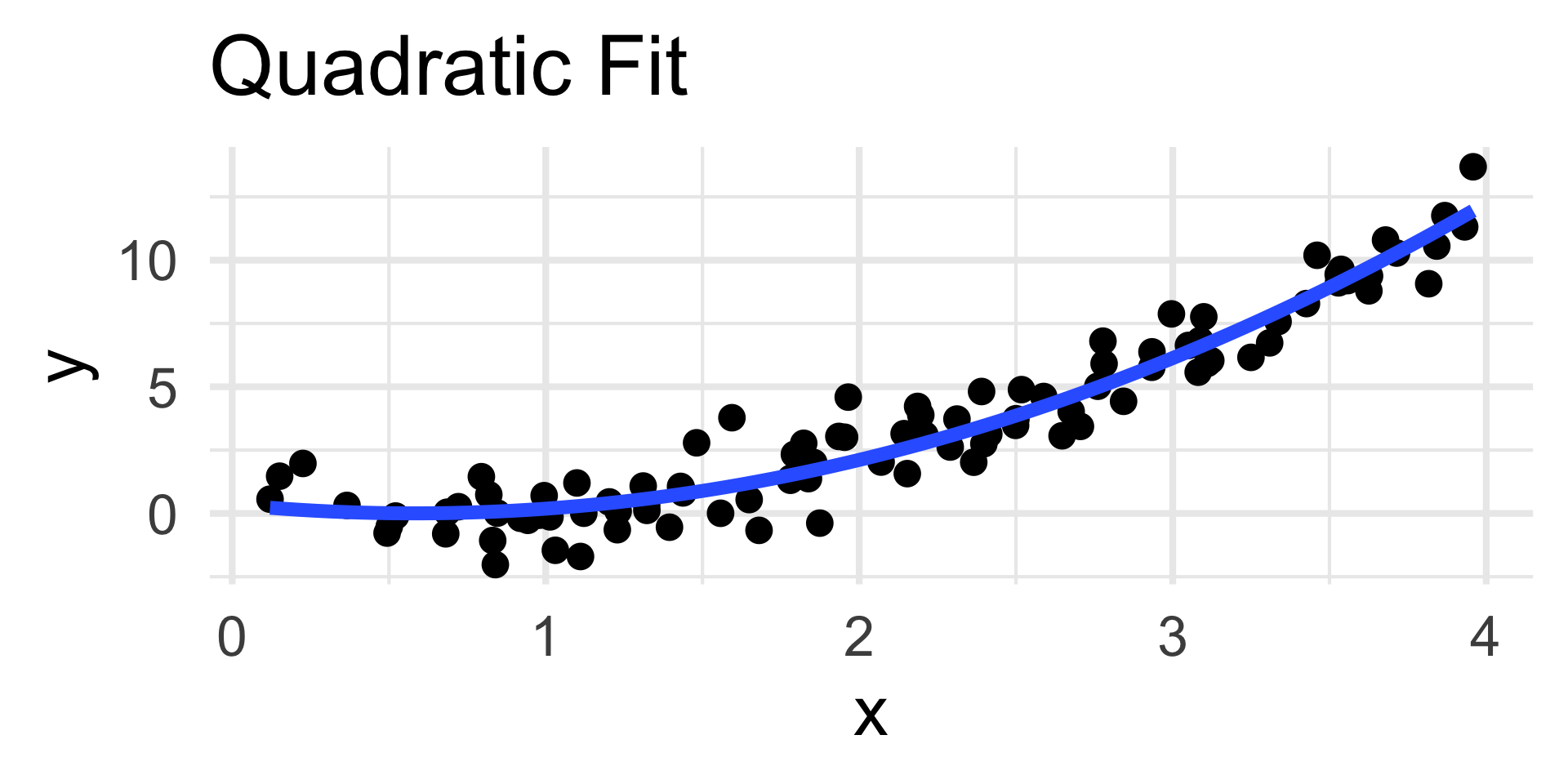
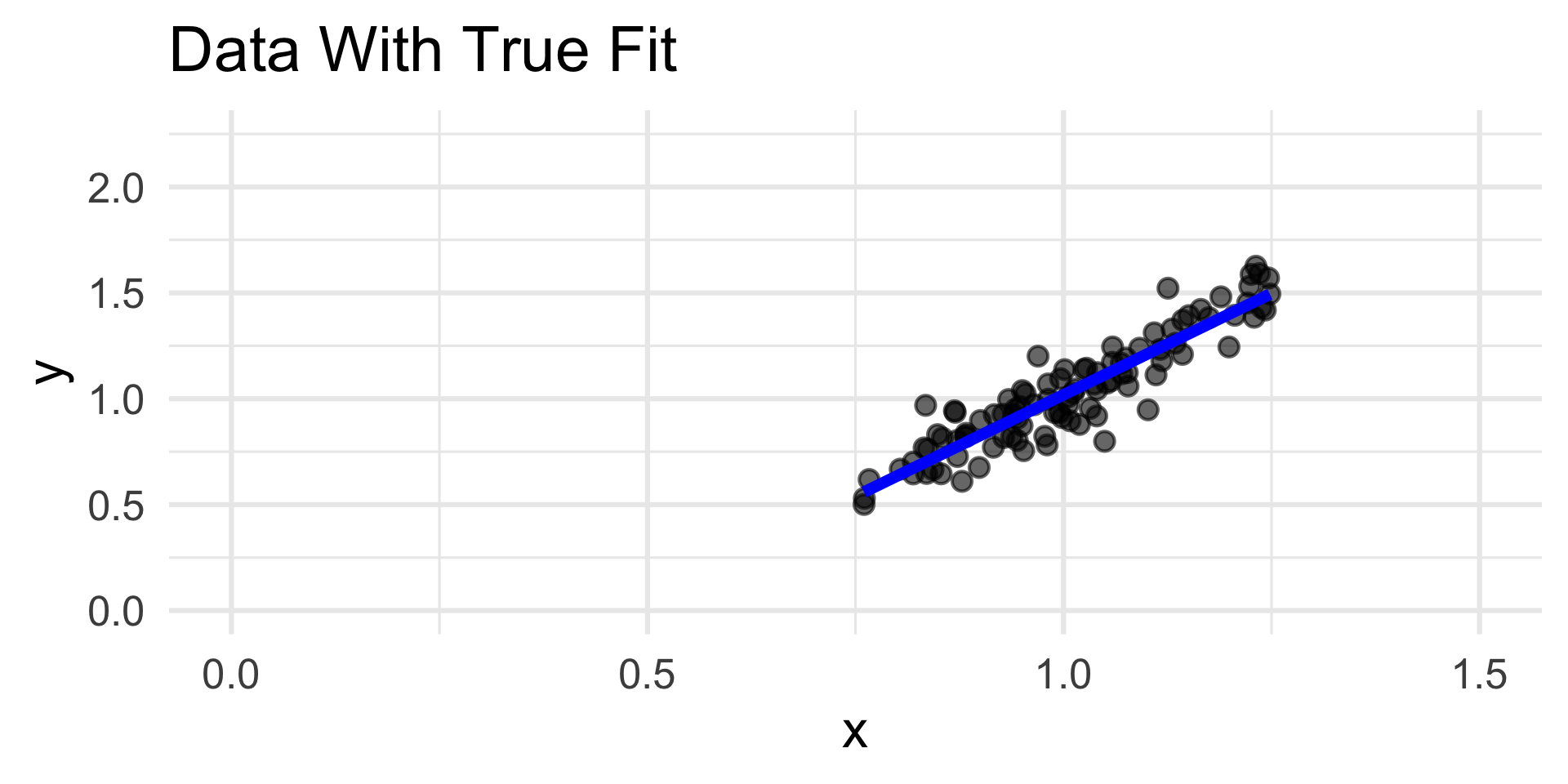
For example, consider the simulated data to the left.
The true relationship appears highly nonlinear; nevertheless, we have fit a linear model to the data.

The coefficients of the linear fit are “optimal” - they minimize risk under squared-error loss!
- In other words, the blue line is the line of best fit to the data.
- But, visually, we believe that this line is not doing a good job of capturing the overall trend in the data.

Model Diagnostics

Residuals

There are a wide variety of tools and techniques that can be used for model diagnostics.
- You’ll learn about some these tools in classes like PSTAT 126 and PSTAT 131/231.
For the purposes of PSTAT 100, we will focus primarily on one specific type of diagnostic tool, known as a residuals plot.
The residuals are defined as \(e_i := y_i - \widehat{y}_i\), where \(\widehat{y}_i\) is the predicted true response (i.e. point along the fitted signal).
- In a sense, they are our attempt at modeling the noise in the data.

Model Diagnostics

Residuals

If our fitted values \(\widehat{y}_i\) capture the signal function perfectly - i.e. if \(\widehat{y}_i = f(x_i)\) for the true signal function \(f(\cdot)\), the residuals becomes \[ e_i = y_i - \widehat{y}_i = (f(x_i) + \varepsilon_i) - f(x_i) = \varepsilon_i \]
That is, if our model is capturing the signal perfectly, then our residuals should behave exactly like noise (which we have assumed is zero mean and possesses constant-variance).
So, the basic idea behind a residuals plot is to plot the residuals, and see how closely they resemble noise!

Model Diagnostics

Residuals

Now, we should be a bit more careful about what we mean by “noise.”
- To that end, let us return to our SLR model: y_i = β₀ + β₁ x_i + ε_i
We make two assumptions about ε_i:
1. Zero-Mean: 𝔼[ε_i] = 0
2. Homoskedasticity: Var[ε_i] = σ², independent of i
Sometimes we will substitute the following assumption in place of the two above: \[ \varepsilon \iid \mathcal{N}(0, \sigma_0^2) \]

Residuals Plots

In a residuals plot, we plot the residuals on the vertical axis and the fitted values on the vertical axis.
A residuals plot indicative of a well-fitting model should display:
- No discernable trend
- Homoskedasticity
On the flipside, a residuals plot missing one or both of these attributes is indicative of a poorly-fitting model.
Let’s take a look at a few examples.

Residuals Plots

Examples

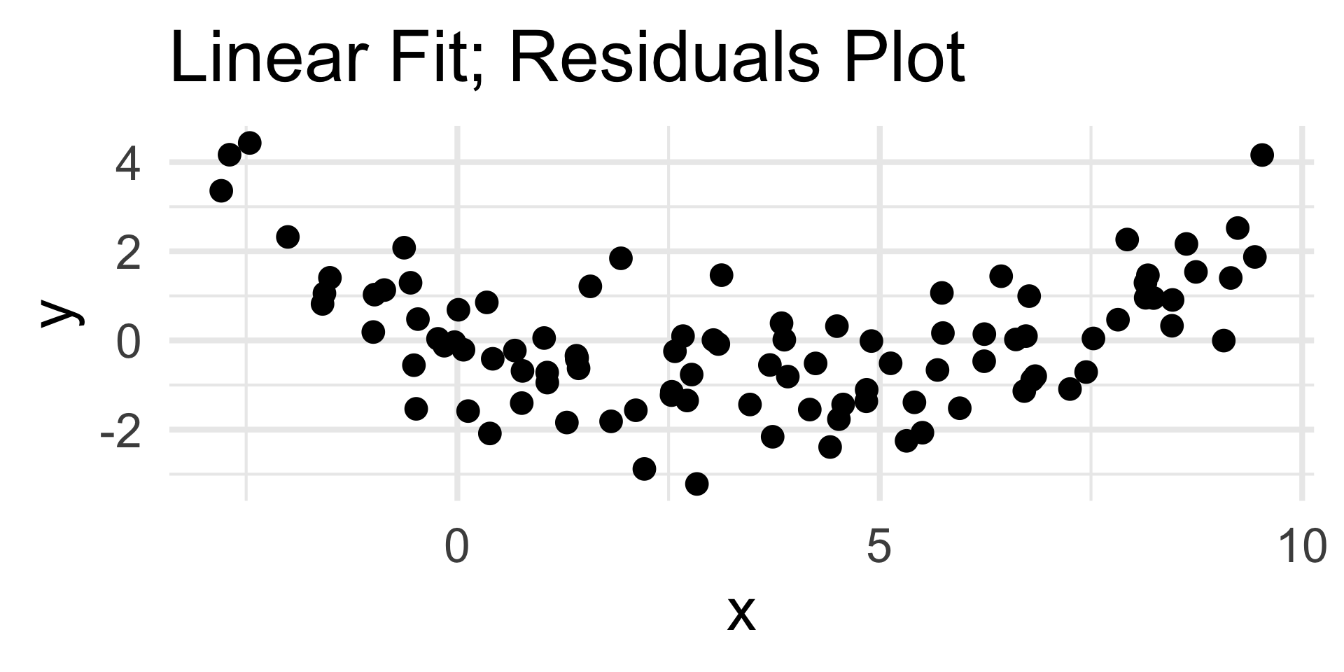
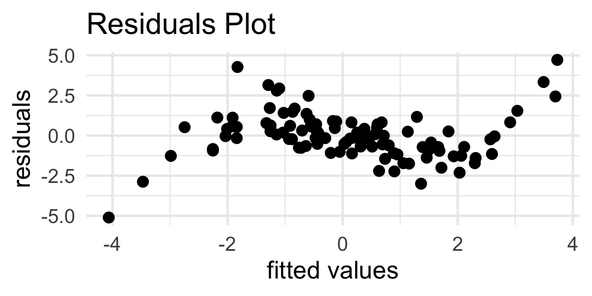
The residuals plot displays a clear quadratic trend, indicating a poor choice of model.
- The scatterplot on the left confirms this.
- Note that the nature of the trend in the residuals plot is indicative of the portion of the model missing; we’ll return to this in a bit.

Residuals Plots

Examples

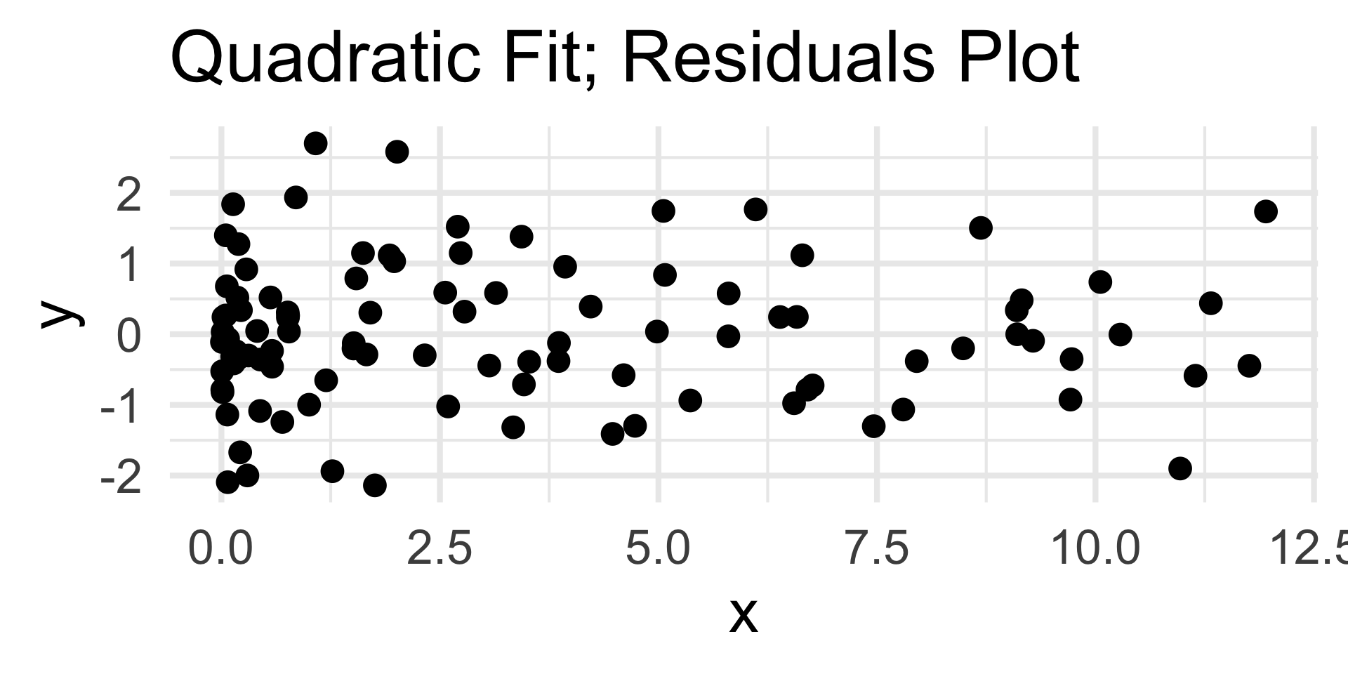
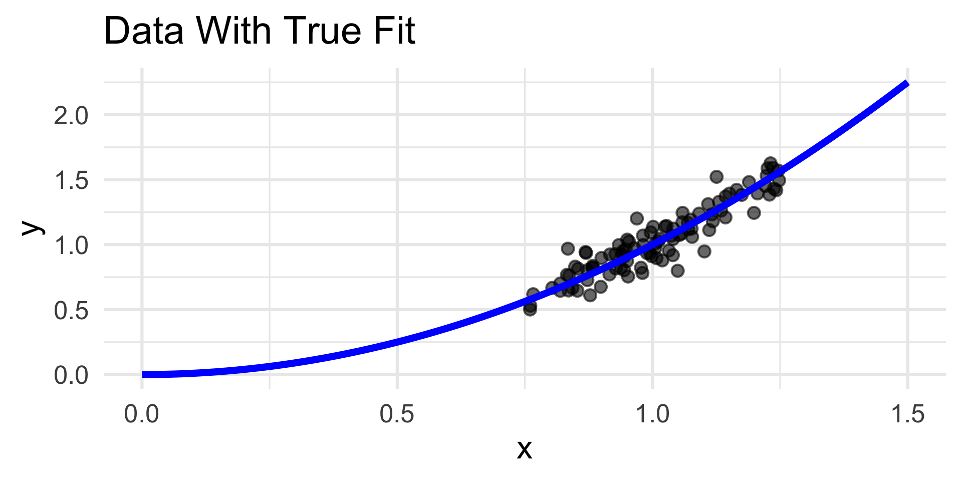
Now, the residuals plot displays no discernable trend along with homoskedasticity.
- This indicates that our choice of quadratic fit was good; certainly in comparison to the linear fit.

Diagnostic 1

Trend in Residuals

As noted, the presence of trend in the residuals plot indicates a poor choice of model.
Indeed, it is not a coincidence that a linear fit to quadratic data displays a quadratic trend in the residuals plot.
Suppose the true model is quadratic: y_i = β₀ + β₁ x_i + β₂ x_i² + ε_i
Further suppose we fit a linear model: ŷ_i = α₀ + α₁ x_i + ε_i
The residuals then take the form: e_i = (β₀ - α₀) + (β₁ - α₁) x_i + β₂ x_i² + ε_i
Even if α₀ matches perfectly with β₀ and α₁ matches perfectly with β₁, the residuals will still have a β₂ x_i² term left over.
- In other words, the expectation of e_i will be quadratic in x.

Misspecified Model

Trend in Residuals

Moral

If the residuals plot displays a trend of the form g(ŷ) for some function g, consider incorporating a term of the form g(x) into the original model.

Your Turn!

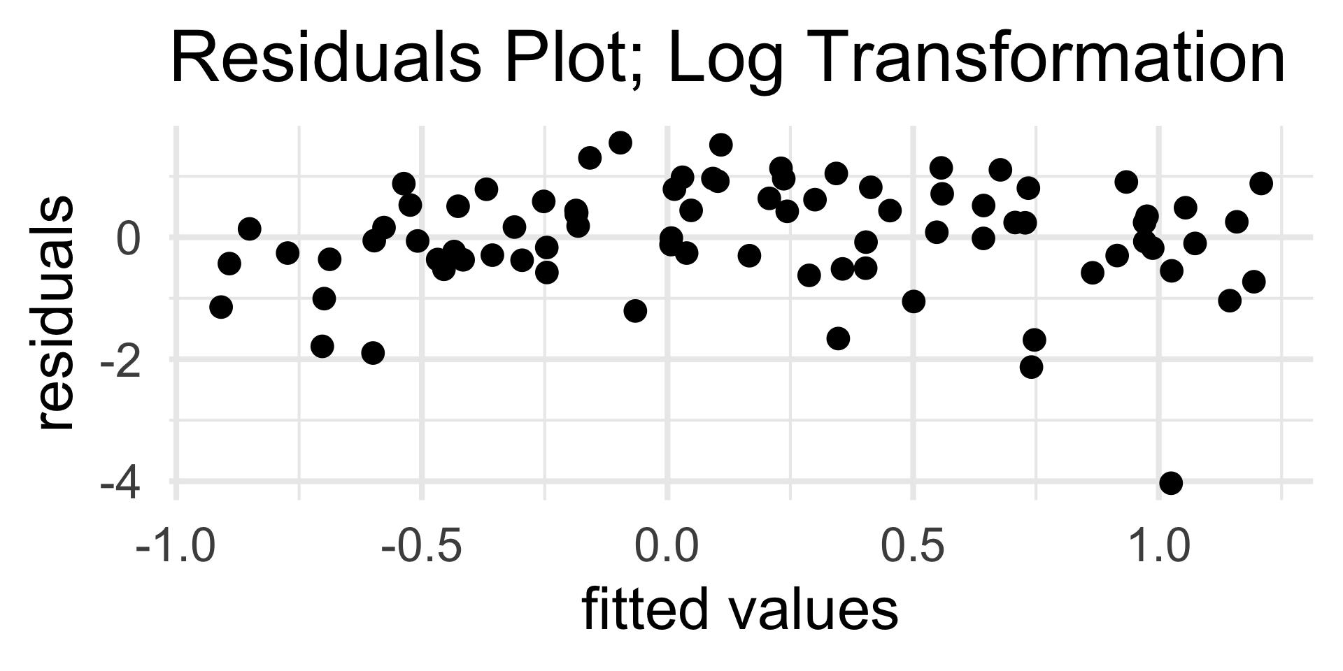
When a simple linear regression model is fit to a particular dataset, the resulting residuals plot is:

Propose an improved model, and justify your choice of improvement.

03:00

Live Demo!

Live Demo!

Using the penguins dataset, let’s fit a linear model of bill depth as a function of body mass; we’ll then generate a residuals plot and decide on whether we believe a linear model was appropriate or not.

Diagnostic 2

Heteroskedasticity in Residuals

The other type of “problem” we might encounter in a residuals graph is heteroksedasticity (i.e. nonconstant variance).
There are a couple of different ways to address heteroskedasticity, most of which I’ll leave for your future PSTAT courses to discuss.
- For the purposes of PSTAT 100, you should just be able to identify the presence of heteroskedasticity from a residuals plot

Why Model?

Prediction

What’s the true (de-noised) bill length (in mm) of a 4000g penguin?

Inference

How confident are we in our guess about the relationship between bill length and body mass?

Prediction: Example

gentoo <- penguins %>% filter(species == "Gentoo")
lm1 <- lm(bill_depth_mm ~  body_mass_g, gentoo)
(y1 <- predict(lm1, newdata = data.frame(body_mass_g = 5010)))

       1 
14.88971

Code

gentoo %>% ggplot(aes(x = body_mass_g, 
                        y = bill_depth_mm)) +
  geom_point(size = 4, alpha = 0.4) + 
  theme_minimal(base_size = 24) +
  annotate("point", shape = 15, x = 5010, y = y1, col = "red", size = 6) +
  xlab("body mass (g)") + ylab("bill depth (mm)") +
  ggtitle("Bill Depth vs. Body Mass", 
          subtitle = "Gentoo Only")

Prediction: Example

For a general statistical model y_i = f (x_i) + ε_i , a prediction for the true response value at an input x is given by first estimating f (either parametrically or nonparametrically) by \(\widehat{f}\), and then returning a fitted value \[ \widehat{y}_i := \widehat{f}(x) \]

Dangers of Extrapolation

Our “optimal” model fit is only optimal for the range of data on which it was fit.
- Extrapolation (predicting based on predictor values far outside the range originally observed) assumes that our proposed model holds even far outside the range of data we initially observed - an assumption that is very dangerous to make.
So, don’t do it!

Dangers of Extrapolation

penguins %>% select(bill_length_mm, body_mass_g) %>% summary()

 bill_length_mm   body_mass_g  
 Min.   :32.10   Min.   :2700  
 1st Qu.:39.23   1st Qu.:3550  
 Median :44.45   Median :4050  
 Mean   :43.92   Mean   :4202  
 3rd Qu.:48.50   3rd Qu.:4750  
 Max.   :59.60   Max.   :6300  
 NA's   :2       NA's   :2

The summary() function provides (among other things) a good way to check the range of covariate (and response) values.

Inference

Let’s now discuss inference on the SLR model.
The OLS estimators (recall the distinction between an estimate and an estimator) are given by \[ \widehat{B}_0 = \overline{Y}_n - \widehat{B}_1 \overline{X}_n; \qquad \widehat{B}_1 = \frac{\sum_{i=1}^{n}(X_i - \overline{X}_n)(Y_i - \overline{Y}_n)}{\sum_{i=1}^{n}(X_i - \overline{X}_n)^2} \]
One can show these are unbiased estimators for the true slope and intercept β₀ and β₁, respectively.
If we assume the errors in the model are normally distributed, one can show that the standardized OLS estimators follow a t_n-2 distribution.

Inference

Regression Tables

Code

x <- rnorm(100)
y <- 0.5 + 1.5*x + rnorm(100)

lm(y ~ x) %>% summary()


Call:
lm(formula = y ~ x)

Residuals:
     Min       1Q   Median       3Q      Max 
-3.06033 -0.54038  0.05607  0.77025  2.02609 

Coefficients:
            Estimate Std. Error t value Pr(>|t|)    
(Intercept)  0.36060    0.10755   3.353  0.00114 ** 
x            1.40672    0.09971  14.109  < 2e-16 ***
---
Signif. codes:  0 '***' 0.001 '**' 0.01 '*' 0.05 '.' 0.1 ' ' 1

Residual standard error: 1.072 on 98 degrees of freedom
Multiple R-squared:  0.6701,    Adjusted R-squared:  0.6667 
F-statistic: 199.1 on 1 and 98 DF,  p-value: < 2.2e-16

This is an example of a regression table.

Inference

Regression Tables

Coefficients:
            Estimate Std. Error t value Pr(>|t|)    
(Intercept)  0.36060    0.10755   3.353  0.00114
x            1.40672    0.09971  14.109  < 2e-16

Estimate
Std. Error
t-Value
Pr(>|t|)

The Estimate column provides the actual OLS estimates, given the data.

The Std. Error column provides the standard errror (i.e. standard deviation) of the OLS estimators, given the data.

The t Value column provides the observed value of \(\widehat{B} / \mathrm{se}(\widehat{B})\), which, assuming the true coefficient is zero, follows a t distribution with (n - 2) degrees of freedom.

Hm… what’s this doing?

Based on this (and perhaps some additional work), what is a 95% confidence interval for the true slope?

Inference

Regression Tables

We saw something like Pr(>|t|) in Lab yesterday. What context was that in, and what did this quantity mean in that context?

lm(y ~ x) %>% coef()

(Intercept)           x 
 0.01144773 -0.10536744

So, according to R, a one-unit increase in x corresponds to a predicted 0.105-unit change in y.
Do we believe this?
- Do we really think there is a trend at all?

Inference

Trend or Not?

Wouldn’t it be nice to statistical test whether or not there even is a linear relationship between the response and covariate?
Thankfully, there is one! Specifically, in the SLR model, which parameter controls/captures the linear relationship between x and y?
So, testing whether or not there is a trend is analogous to testing the null H₀: β₁ = 0 against the alternative H_A: β₁ ≠ 0.
This is why the sampling distributions of the OLS estimators is useful - it allows us to construct a hypothesis test for whether or not a linear association exists between x and y.

Inference

Trend or Not?

The final column in the regression table provides a p-value for the test of H₀: β₁ = 0 against the two-sided alternative H_A: β₁ ≠ 0.

lm(y ~ x) %>% summary()


Call:
lm(formula = y ~ x)

Residuals:
     Min       1Q   Median       3Q      Max 
-2.05195 -0.43265 -0.07854  0.48583  1.93858 

Coefficients:
            Estimate Std. Error t value Pr(>|t|)
(Intercept)  0.01145    0.07929   0.144    0.885
x           -0.10537    0.07807  -1.350    0.180

Residual standard error: 0.7929 on 98 degrees of freedom
Multiple R-squared:  0.01825,   Adjusted R-squared:  0.008229 
F-statistic: 1.821 on 1 and 98 DF,  p-value: 0.1803

Next Time

Tomorrow, we’ll start generalizing from only one covariate to multiple covariates.
- This is going to involve some linear algebra!
We’ll also get some hands-on practice with the R side of regression, and further practice with interpreting results.
Reminder: please don’t forget to turn in HW02 this sunday!

PSTAT 100: Lecture 14

Recap

Statistical Modeling

Recap

Types of Statistical Models

Penguins

An Example

Penguins

An Example

Penguins

Step 1: Propose a Model

Simple Linear Regression Model

Step 1: Propose a Model

Simple Linear Regression Model

As Applied to the Palmerpenguins Dataset

Simple Linear Regression Model

Step 2: Fit the Model to the Data

Simple Linear Regression Model

Step 2: Fit the Model to the Data

Simple Linear Regression

Step 2: Estimate Parameters

Simple Linear Regression

Step 2: Estimate Parameters

Simple Linear Regression

Empirical Verification

Penguins

The Fitted SLR Model

Model Diagnostics

Model Diagnostics

Example: Poor Choice of Model

Model Diagnostics

Residuals

Model Diagnostics

Residuals

Model Diagnostics

Residuals

Residuals Plots

Residuals Plots

Examples

Residuals Plots

Examples

Diagnostic 1

Trend in Residuals

Misspecified Model

Trend in Residuals

Live Demo!

Diagnostic 2

Heteroskedasticity in Residuals

Why Model?

Prediction: Example

Prediction: Example

Dangers of Extrapolation

Dangers of Extrapolation

Inference

Inference

Regression Tables

Inference

Regression Tables

Inference

Regression Tables

Inference

Trend or Not?

Inference

Trend or Not?

Next Time

As Applied to the `Palmerpenguins` Dataset