PSTAT 100: Lecture 13
Examples of Statistical Modeling
Density Estimation
Framework
Data: A collection of numerical values; \(\vect{x} = (x_1, \cdots, x_n)\) we believe to be a realization of an i.i.d. random sample \(\vect{X} = (X_1, \cdots, X_n)\) taken from a distribution with density f().
Goal: to estimate the true value of f() at each point.
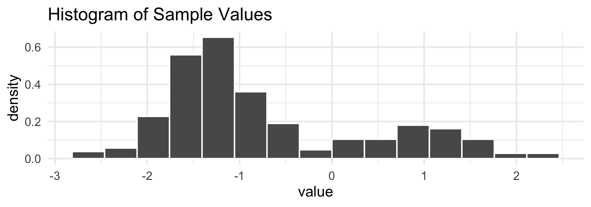
Histograms, Revisited

Histograms, Revisited
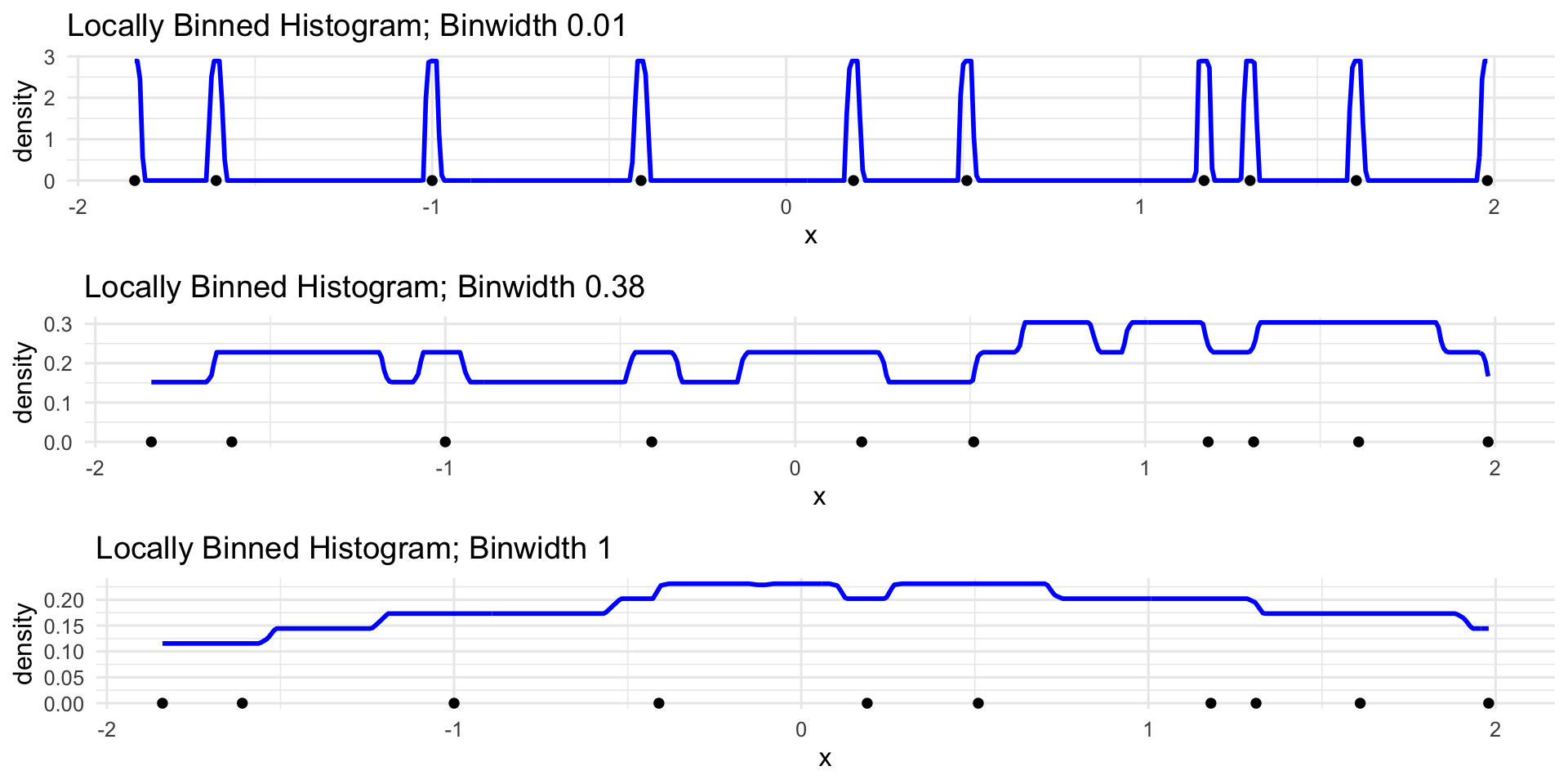
Local Binning
\[ \widehat{f}_{\mathrm{lb}}(x) = \frac{1}{nh} \sum_{i=1}^{n} 1 \! \! 1_{\{ \left| x_i - x \right| < \frac{h}{2} \}} \]

Histograms, Revisited
Local Binning
Histograms, Revisited
Local Binning
\[ \widehat{f}_{\mathrm{lb}}(x) = \frac{1}{n} \sum_{i=1}^{n} \left[ \frac{1}{h} 1 \! \! 1_{\{ \left| x_i - x \right| < \frac{h}{2} \}} \right] \]

- Changing xi amounts to changing the “center” of the “box”
- Changing h amounts to changing the width and height of the “box”
- Note, however, that for any value of h and xi, the area underneath this graph is always 1.
- Nonnegative function that integrates to one…
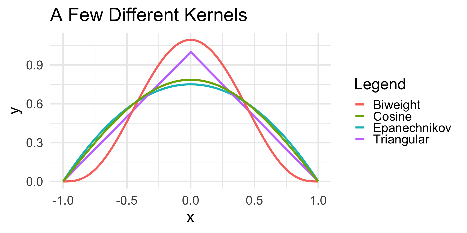
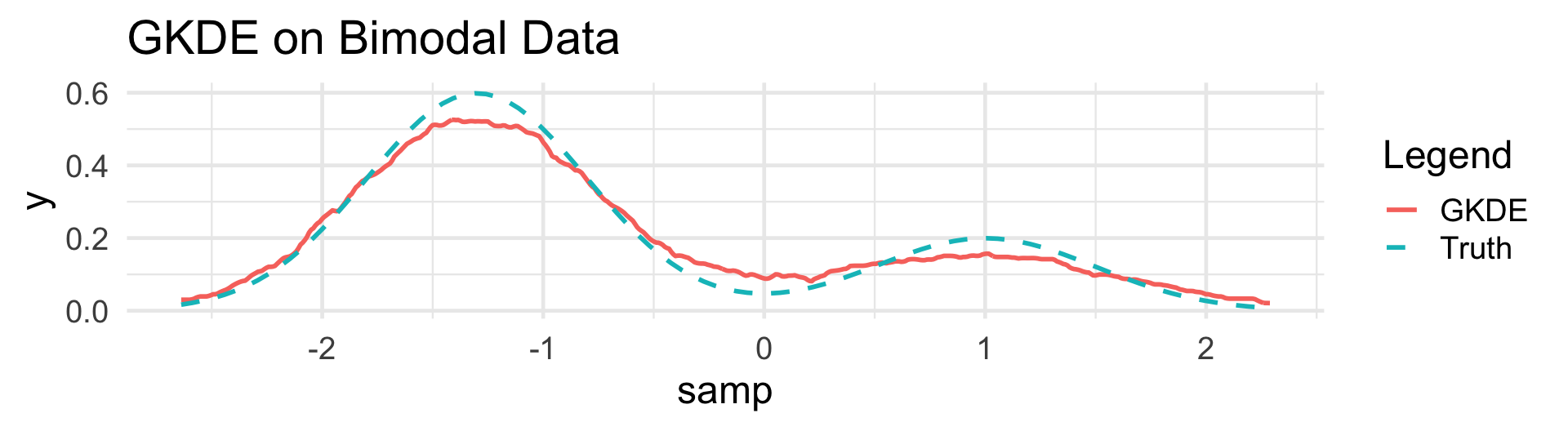
Kernel Density Estimation
Kernels
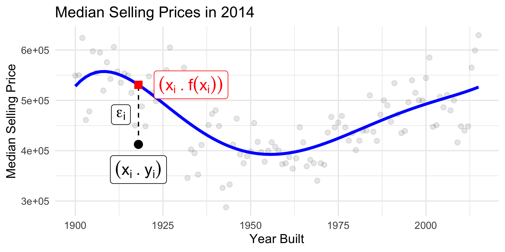
Loss Functions
There are many choices for loss functions, each with pros and cons.
For numerical data, the two most common loss functions are:
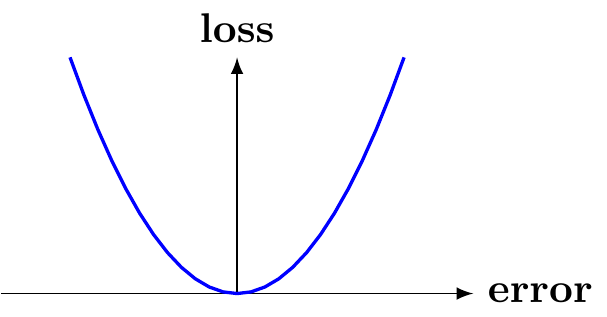
Squared Error (aka L2)
\(\mathcal{L}(y_i, \theta) = (y_i - \theta)^2\)
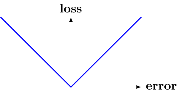
Absolute Error (aka L1)
\(\mathcal{L}(y_i, \theta) = |y_i - \theta|\)
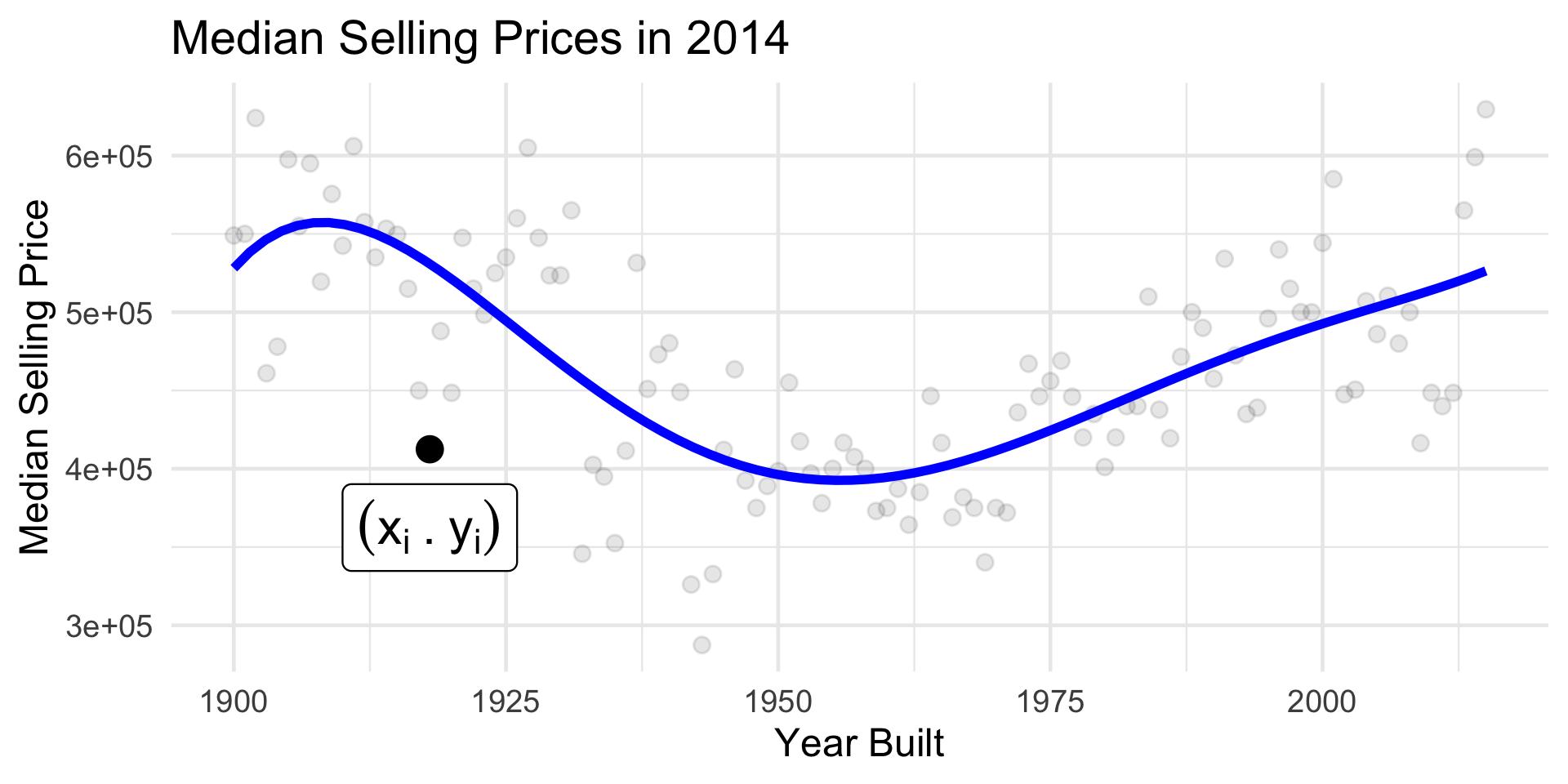
Housing Data
An Example
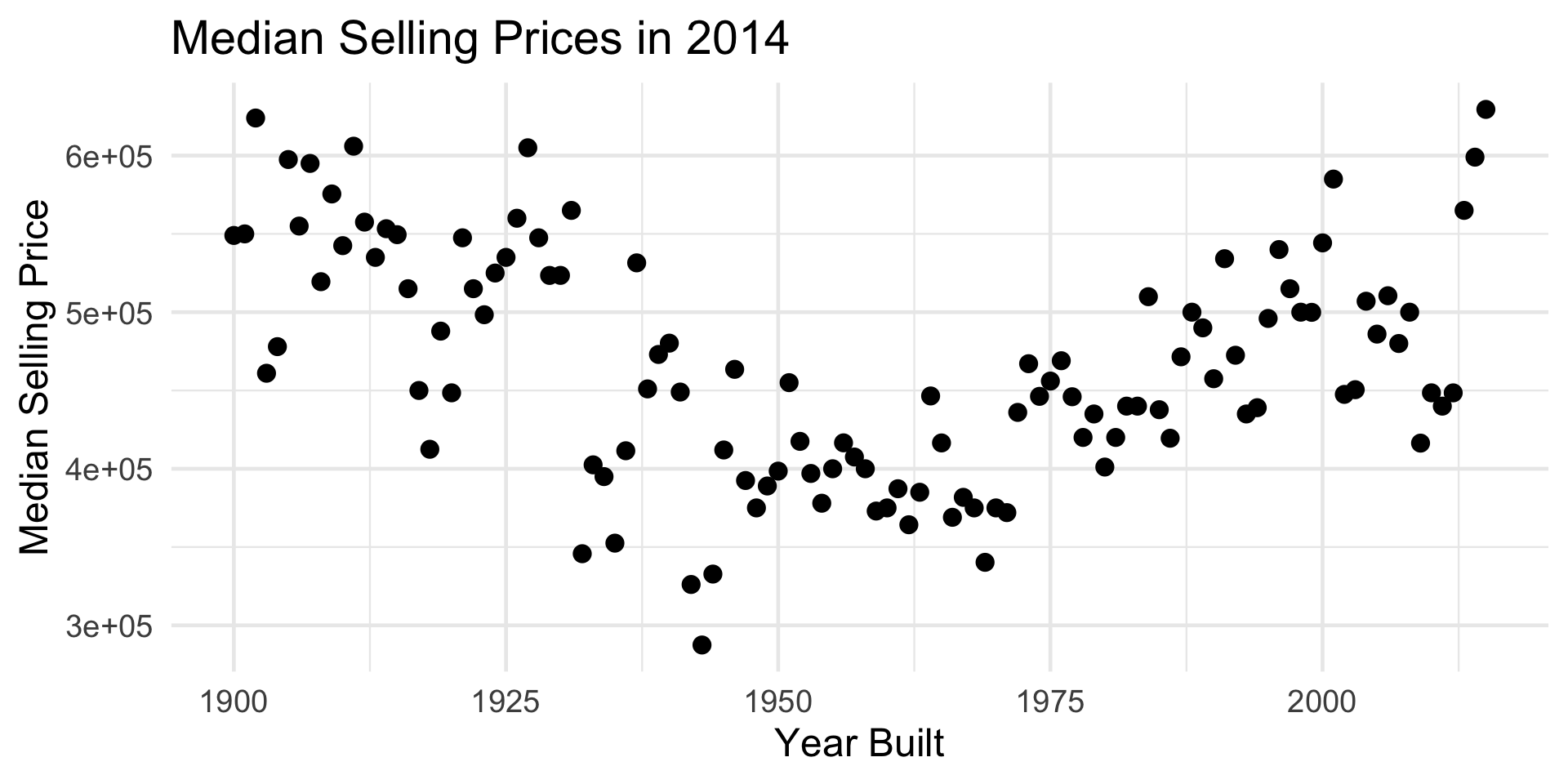
Housing Data
Building a Model
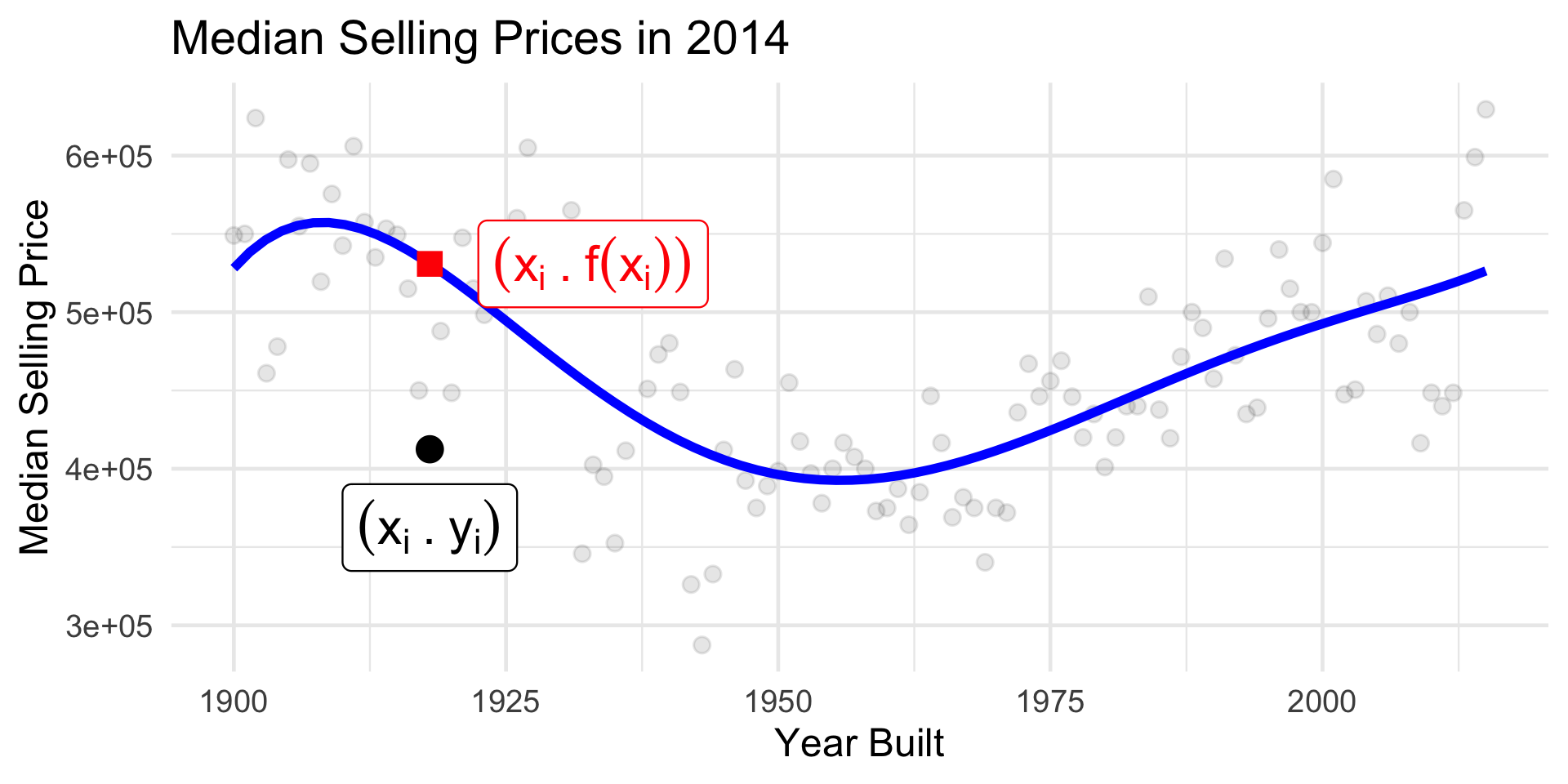
Housing Data
Building a Model
Housing Data
Building a Model
Housing Data
Building a Model
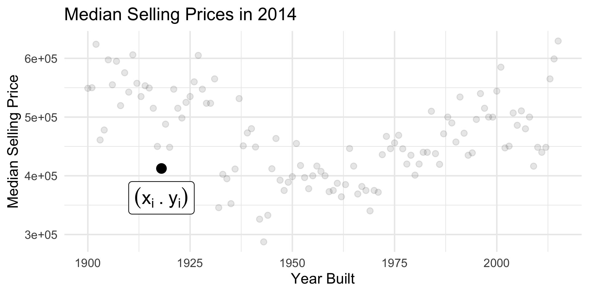
Why Model?
Prediction
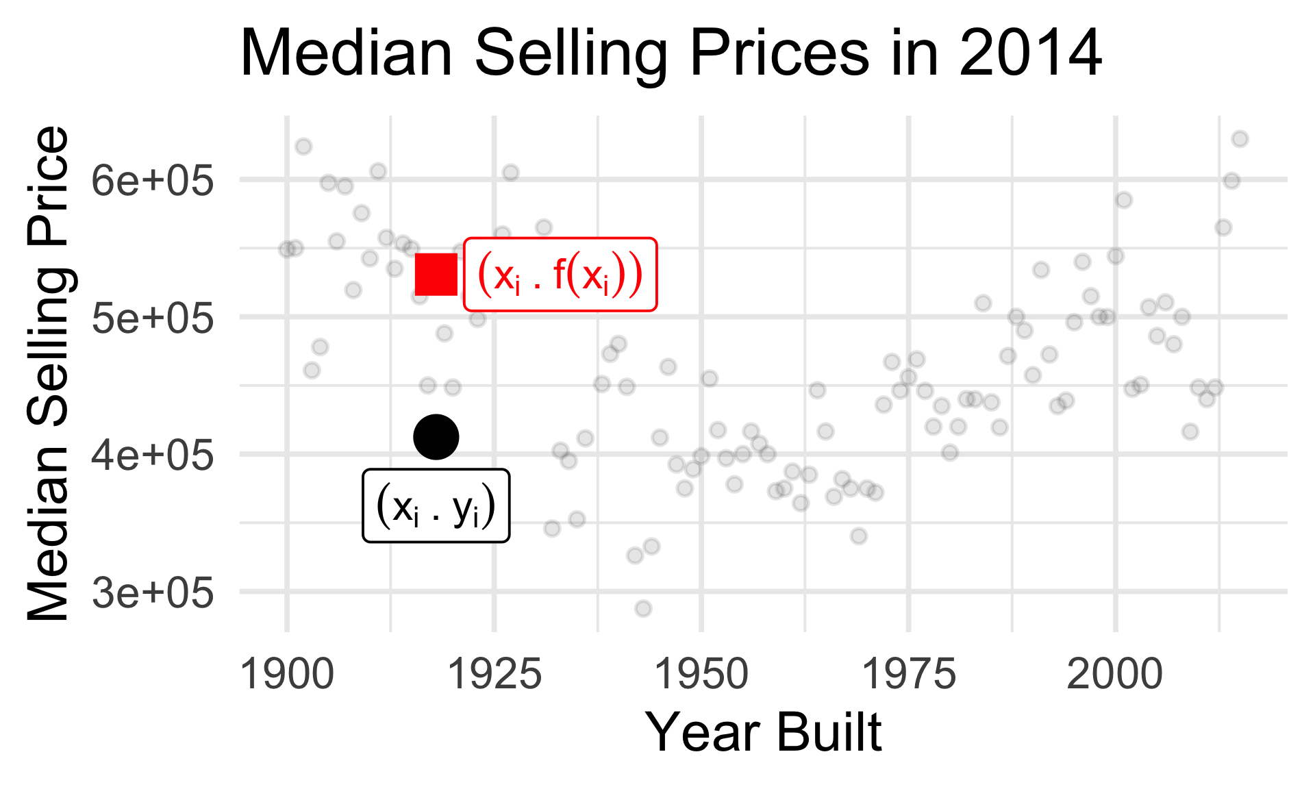
- What’s the true (de-noised) median selling price of a house built in 1918?
Inference
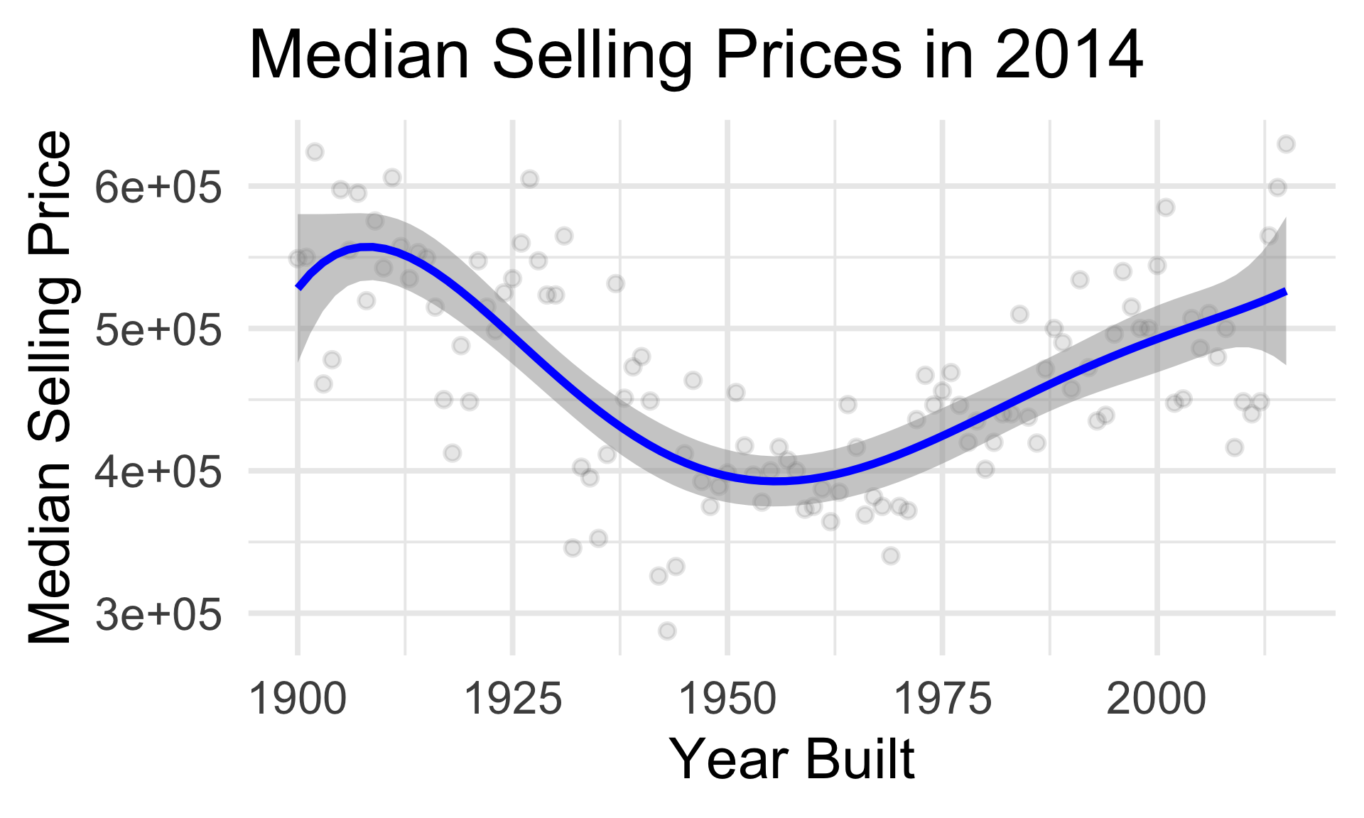
- How confident are we in our guess about the relationship between year built and selling price?