PSTAT 100: Lecture 11
Hypothesis Testing
Recap
General Framework for Inference

We have a population, governed by a set of population parameters that are unobserved (but that we’d like to make claims about).
To make claims about the population parameters, we take a sample.
We then use our sample to make inferences (i.e. claims) about the population parameters.
- Inference could mean estimation or hypothesis testing
Cats - Again!
Toe Beans…
- According to a Quora post, the average cat has about a 10% chance of being born with polydactyly

Polydactyly refers to a condition whereby an animal is born with extra digits (e.g. extra fingers in humans, extra toes in cats, etc.)
Suppose we wish to assess the validity of the Quora claim, using data.
- Note that we’re not necessarily trying to estimate the true incidence of polydactyly among cats!
Polydactyly Example
Code
pop <- read.csv("cats_pop.csv") %>% unlist()
set.seed(100)

props <- c()
for(b in 1:1000){
  temp_samp <- sample(pop, size = 2500)
  props <- c(props, ifelse(temp_samp == "poly", 1, 0) %>% mean())
}

data.frame(x = props) %>% ggplot(aes(x = x)) +
  geom_histogram(aes(y = after_stat(density)), bins = 13, col = "white") +
  theme_minimal(base_size = 18) +
  ggtitle("Histogram of Sample Proportions",
          subtitle = "1000 samples of size 2500") +
  xlab("sample proportion")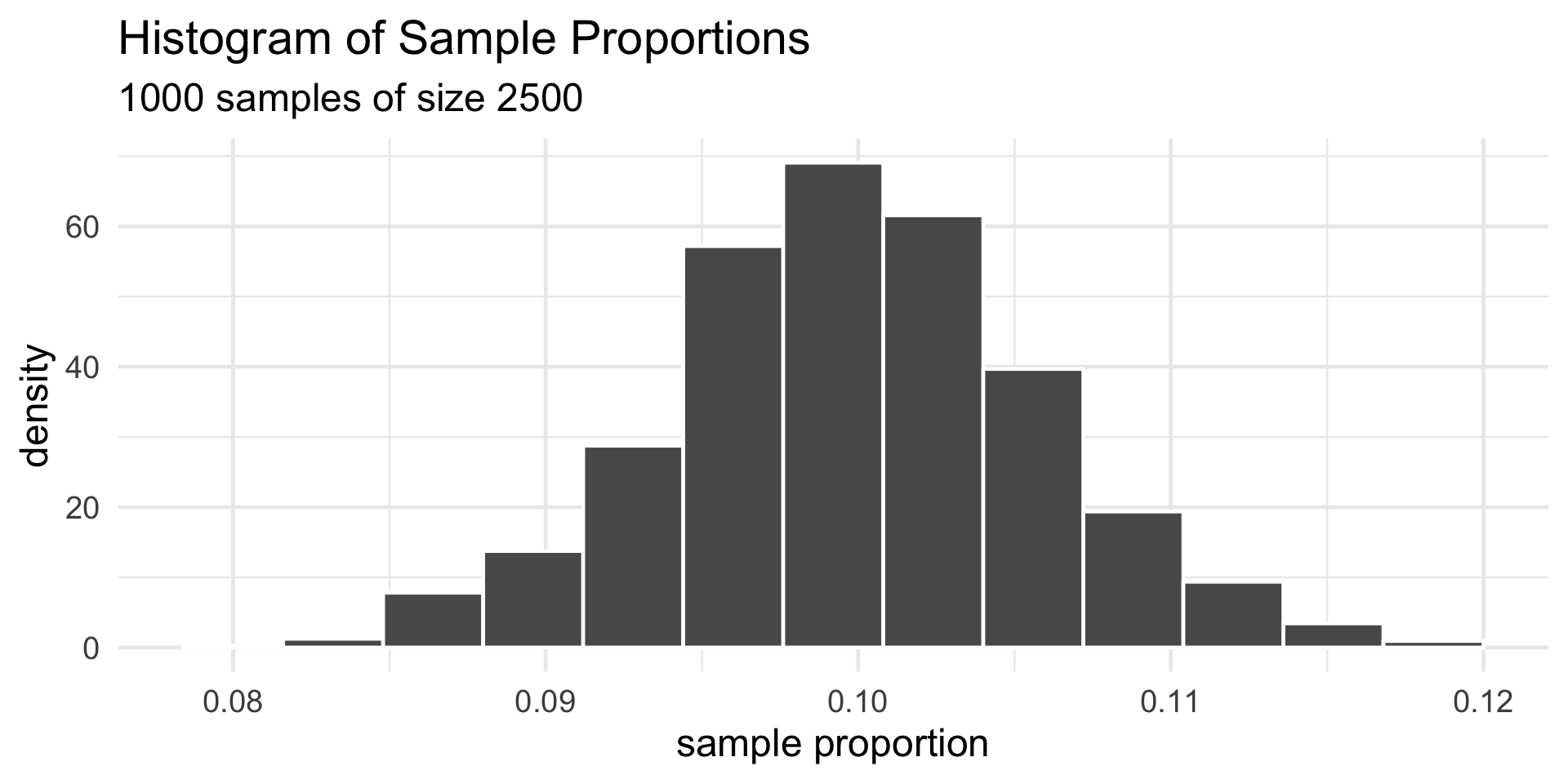
Polydactyly Example
Code
data.frame(x = props) %>% ggplot(aes(x = x)) +
  geom_histogram(aes(y = after_stat(density)), bins = 13, col = "white") +
  theme_minimal(base_size = 18) +
  ggtitle("Histogram of Sample Proportions",
          subtitle = "1000 samples of size 2500") +
  xlab("sample proportion") +
  stat_function(fun = dnorm,
                args =
                  list(
                    mean = mean(pop == "poly"),
                    sd = sqrt(mean(pop == "poly") * (1 - mean(pop == "poly")) / 2500)
                  ),
                col = "blue", linewidth = 1.5
              )
Hypothesis Test for a Proportion

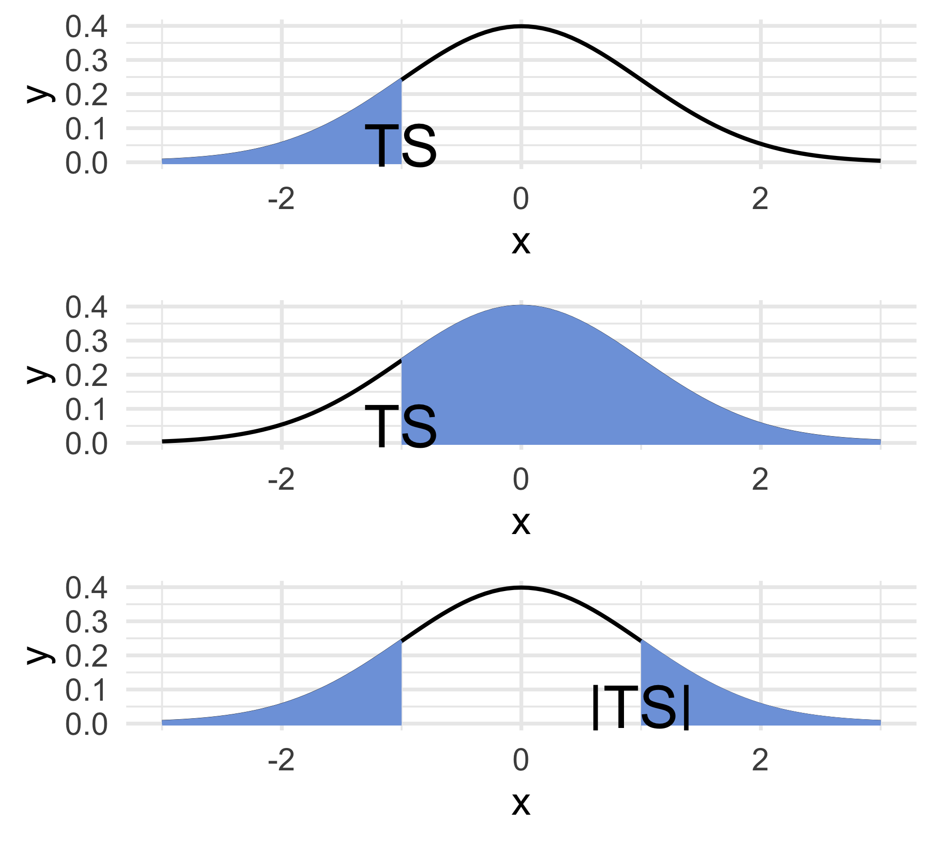
- The curve represents the density of the test statistic, under the null.
- By construction, the shaded areas must together equal α.
Therefore, the equation we have is \[ 2[1 - \Phi(k)] = \alpha \ \implies \ \boxed{k = \Phi^{-1}\left( 1 - \frac{\alpha}{2} \right)}\]
Remember, we set the value of α at the beginning, to some small number.
- Some common significance levels are 0.01, 0.05, and 0.1, though certain contexts may require smaller or higher levels of significance.
p-Values
Instead of phrasing our test in terms of critical values, we can equivalently formulate things in terms of what is known as a p-value.
The p-value of an observed value of a test statistic is the probability, under the null, of observing something as or more extreme (in the direction of the alternative) as what was observed.
- Lower-tailed: ℙ(TS < ts)
- Upper-tailed: ℙ(TS > ts)
- Two-sided: ℙ(|TS| > ts)
- Again, draw a picture!