PSTAT 100: Lecture 10

Estimation, Confidence Intervals, and Resampling

Ethan P. Marzban

Department of Statistics and Applied Probability; UCSB

Summer Session A, 2025

\[ \newcommand{\Prob}{\mathbb{P}} \newcommand\R{\mathbb{R}} \newcommand{\N}{\mathbb{N}} \newcommand{\E}{\mathbb{E}} \newcommand{\Prob}{\mathbb{P}} \newcommand{\F}{\mathcal{F}} \newcommand{\1}{1\!\!1} \newcommand{\comp}[1]{#1^{\complement}} \newcommand{\Var}{\mathrm{Var}} \newcommand{\SD}{\mathrm{SD}} \newcommand{\vect}[1]{\vec{\boldsymbol{#1}}} \newcommand{\Cov}{\mathrm{Cov}} \newcommand{\iid}{\stackrel{\mathrm{i.i.d.}}{\sim}} \]

Recap: Statistical Inference

• Yesterday we talked about the general framework of statistical inference.

• We have a population, governed by a set of population parameters that are unobserved (but that we’d like to make claims about).

• To make claims about the population parameters, we take a sample.

• We then use our sample to make inferences (i.e. claims) about the population parameters.

Recap: Statistical Inference

• A function of the random sample is an estimator
  • This is a random quantity; “if I were to take a sample, …”
• The corresponding function of the observed instance (aka realization) of the sample is called an estimate
  • This is a deterministic quantity; “given this particular sample I took, …”

Recap: Statistical Inference

• The sampling distribution of an estimator is simply its distribution.

• For example, we saw that the sampling distribution of the sample mean, assuming a normal population, is normal with mean equal to the population mean and variance equal to the population variance divided by the sample size.

  • We further saw that, thanks to the Central Limit Theorem, this also holds if the population is not normal but the sample size is relatively large.

• Let’s consider one more scenario: suppose \(Y_1, \cdots, Y_n\) represents an i.i.d. sample from the \(\mathcal{N}(\mu, \sigma^2)\) distribution where both µ and σ² are unknown.

  • Note that this differs from the situation we discussed yesterday, in which I had explicitly specified a value for σ².

Sampling Distributions

Sample Mean: Non-Normal Population; Unknown Variance

• As mentioned yesterday, a natural estimator for the population variance is the sample variance, defined as \[ S_n^2 := \frac{1}{n - 1} \sum_{i=1}^{n} (Y_i - \overline{Y}_n)^2 \] and a natural estimator for the population standard deviation is just \(S_n := \sqrt{S_n^2}\).

• Let’s take a look at the sampling distribution of \[ U_n := \frac{\sqrt{n}(\overline{Y}_n - \mu)}{S_n} \]

Sampling Distributions

Sample Mean: Non-Normal Population; Unknown Variance

set.seed(100)    ## for reproducibility
n <- 10          ## sample size
B <- 1000        ## number of samples

u_10 <- c()
for(b in 1:B){
  temp_samp <- rnorm(n)   ## sample from standard normal
  u_10 <- c(u_10, mean(temp_samp) / sd(temp_samp))
}

Sampling Distributions

Sample Mean: Non-Normal Population; Unknown Variance

• Hm… the bulk of this histogram looks normal, but there are some unusually extreme values that we wouldn’t expect to see if \(U_n\) were truly normally distributed.

• Indeed, to check whether a set of values are normally distributed, we often generate a QQ-Plot in which we plot the quantiles of our data against the theoretical quantiles of a normal distribution.

  • If the resulting graph is close to a perfect line, we know the quantiles match and our data is likely to be normally-distributed.
  • Equivalently, if we see marked deviation from linearity in the tails of the plot, we have reason to believe our data is not normally-distributed.

Sampling Distributions

Sample Mean: Non-Normal Population; Unknown Variance

data.frame(u_10) %>% ggplot(aes(sample = u_10)) +
  geom_qq(size = 4) + ggtitle(bquote("Normal QQ-Plot of"~U[n])) +
  geom_qq_line(col = "blue", linewidth = 1.25) +
  theme_minimal(base_size = 18)

Sampling Distributions

Sample Mean: Non-Normal Population; Unknown Variance

• As we see, there are significant deviations from linearity in the tails of the QQ-plot.

• Hence, we conclude that \(U_n\) is not normally-distributed.

  • That is, when we estimate the sample variance, the sampling distribution of the sample mean is no longer normal.

• There is a theoretical result to back up this claim.

Sampling Distributions

Sample Mean: Non-Normal Population; Unknown Variance

Sampling Distribution of Mean; Estimated Variance

Given an i.i.d. sample (Y₁, …, Y_n) from a distribution with finite mean µ and finite variance σ², \[ \frac{\sqrt{n}(\overline{Y}_n - \mu)}{S_n} \stackrel{\cdot}{\sim} t_{n - 1} \] where \(S_n := \sqrt{(n - 1)^{-1} \sum_{i=1}^{n} (Y_i - \overline{Y}_n)^2}\) and \(t_{n - 1}\) denotes the t-distribution with ν degrees of freedom.

• You will discuss the t-distribution further in PSTAT 120B. For our purposes, just note that the t-distribution looks a lot like a standard normal distribution but with wider tails.

Sampling Distributions

The t Distribution

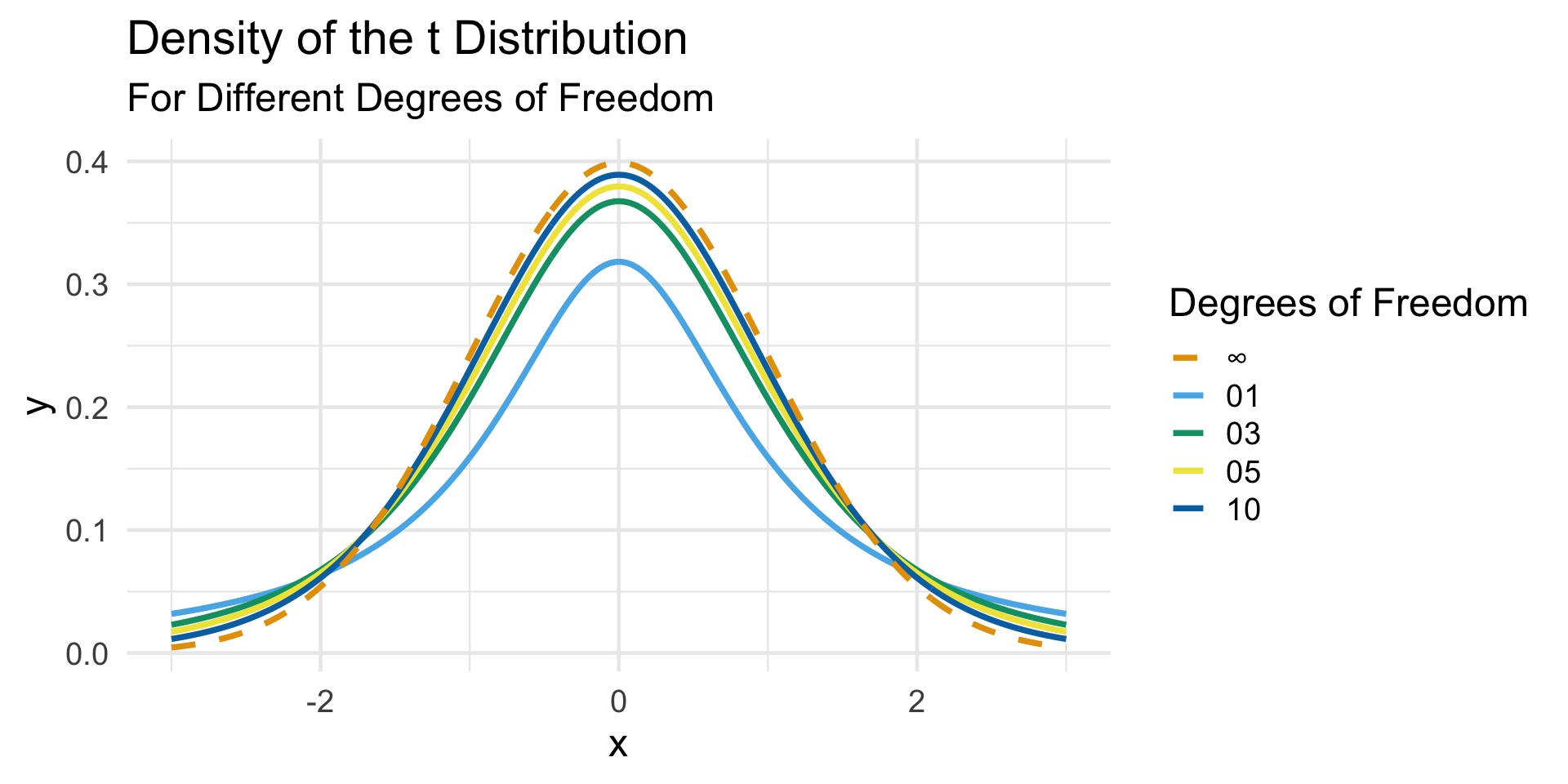
Sampling Distributions

Sample Mean: Non-Normal Population; Unknown Variance

data.frame(u_10) %>% ggplot(aes(sample = u_10)) +
  geom_qq(size = 4, distribution = stats::qt, dparams = 9) + 
  ggtitle(bquote(t[9]~"QQ-Plot of"~U[n])) +
  geom_qq_line(col = "blue", , distribution = stats::qt, dparams = 9,
               linewidth = 1.25) +
  theme_minimal(base_size = 18)

Confidence Intervals

Leadup

• All of the estimators we considered thus far (sample mean, sample variance) are examples of point estimators; they reduce the sample to a single point.

• In some cases, however, a point estimator may be too restrictive.

• To borrow an analogy from OpenIntro Statistics (an introductory stats textbook I highly recommend!):

Using only a point estimate is like fishing in a murky lake with a spear. We can throw a spear where we saw a fish, but we will probably miss. On the other hand, if we toss a net in that area, we have a good chance of catching the fish. (pg. 181)

Confidence Intervals

• The statistical analog of using a net is using a confidence interval.

• Loosely speaking, a confidence interval is an interval that we believe, with some degree of certainty (called the coverage probability), covers the true value of the parameter of interest.

• For example, we are 100% certain that the true average weight of all cats in the world is somewhere between 0 and ∞; therefore, a 100% confidence interval for µ (the true average weight of all cats in the world) is [0, ∞).

• However, consider the interval [5, 20]. Are we 100% certain that the true average weight of all cats in the world is between 5 and 20 lbs? Probably not; so, the associated coverage probability of the interval [5, 20] is smaller than 100%.

Confidence Intervals

• When constructing a Confidence Interval (CI), we often start with a coverage probability in mind first.

• Some common coverage probabilities are: 90%, 95%, and 99%.

  • This isn’t to say other coverage probabilities are never used; given domain knowledge, it may be desired to use a different coverage probability.

• Suppose we wish to construct a p CI for the mean; i.e. given a population with (unknown) mean µ, we wish to construct a CI with coverage probability p (e.g. 0.95).

Confidence Intervals for the Mean

• It seems natural to start with \(\overline{Y}_n\), the sample mean. Indeed, we’ll first take our CI to be of the form \[ \overline{Y}_n \pm \mathrm{m.e.} \] for some margin of error \(\mathrm{m.e.}\).
  • We can think of this as saying: “I think the sample mean is probably a good guess for the population mean. However, I acknowledge there is sampling variability, and I should include some padding in my estimate.”
• With this interpration, we see that the margin of error should depend on two things:
  • The coverage probability p (higher p implies what about the margin of error?)
  • The variance of \(\overline{Y}_n\) (to capture variability between samples).

Confidence Intervals for the Mean

• So, let’s just take the margin of error to be the product of two terms: the variance of \(\overline{X}_n\), and a confidence coefficient c (a value related to our coverage probability p): \[ \overline{Y}_n \pm c \cdot \frac{\sigma}{\sqrt{n}} \]

• So, all that’s left is to figure out what the confidence coefficient c should be.

• Indeed, we should select it such that \[ \Prob\left( \overline{Y}_n - c \cdot \frac{\sigma}{\sqrt{n}} \leq \mu \leq \overline{Y}_n + c \cdot \frac{\sigma}{\sqrt{n}} \right) = p \]

Confidence Intervals for the Mean

• Equivalently, \[ \Prob\left( -c \leq \frac{\sqrt{n}(\overline{Y}_n - \mu)}{\sigma} \leq c \right) = p \]

• Hey- I know the sampling distribution of the middle quantity (provied we either have a normally-distributed population, or a large enough sample size for the CLT to kick in)!

• So, our equivalent condition c must satisfy is \[ 2 \Phi(c) - 1 = p \ \implies \ c = \Phi^{-1}\left( \frac{1 + p}{2} \right) \]

Confidence Intervals for the Mean

CI for the Mean; Known Variance

Suppose (Y₁, …, Y_n) represents an i.i.d. sample from a distribution with finite mean µ and known variance σ² < ∞. If either the Y_i’s are known to be normally distributed or the sample size n is large (n ≥ 30), a p confidence interval for µ is given by \[ \overline{Y}_n \pm \Phi^{-1}\left( \frac{1 + p}{2} \right) \cdot \frac{\sigma}{\sqrt{n}}\]

• For example, the confidence coefficient associated with a 95% interval for the mean is given by

qnorm((1 + 0.95) / 2)

[1] 1.959964

Confidence Intervals for the Mean

CI for the Mean; Unknown Variance

Suppose (Y₁, …, Y_n) represents an i.i.d. sample from a distribution with finite mean µ and unknown variance σ² < ∞. If either the Y_i’s are known to be normally distributed or the sample size n is large (n ≥ 30), a p confidence interval for µ is given by \[ \overline{Y}_n \pm F_{t_{n - 1}}^{-1} \left( \frac{1 + p}{2} \right) \cdot \frac{S_n}{\sqrt{n}}\] where \(F_{t_{n - 1}}^{-1}(\cdot)\) denotes the inverse CDF of the t_n-1 distribution.

• For example, the confidence coefficient associated with a 95% interval for the mean, given a sample size of 32, is given by

qt((1 + 0.95) / 2, 31)

[1] 2.039513

Your Turn!

Your Turn!

A consultant from the EPA (Environmental Protection Agency) is interested in estimating the average CO₂ emissions among all US households. To that end, they collect a sample of 35 US households; the average emissions of these 35 households is 9.13 mt/yr and the standard deviation of these emissions is 2.43 mt/yr. Construct a 90% confidence interval for the true average CO₂ emissions among all US households using the consultant’s data.

Caution

You’ll need a computer for this one!

05:00

Resampling Methods

Leadup

• Much of our discussion yesterday and today has been simulation-based: for instance, yesterday we repeatedly sampled from the Exponential distribution and constructed the empirical sampling distribution for the sample mean.
  • Furthermore, in our simulations, we sampled directly from the population.
• What happens if we don’t have access to the population distribution?
  • For example, suppose we have 100 cat weights, but we don’t want to necessarily assume that the weight of a randomly-selected cat follows the normal distribution.

Resampling Methods

• Here is an idea: what if we treat this sample as the population itself?

  • If we do, we can simply generate as many samples (with replacement) as we like and still construct empirical sampling distributions for estimators using the procedure we implemented yesterday.

• This is the idea behind the bootstrap, which itself belongs to a class of techniques known as resampling methods.

• Let’s run through an example together.

• Imagine we have a vector of 100 cat weights, stored in a variable called cat_wts.

Bootstrapping: Example

head(cat_wts)

[1]  8.893 10.921 10.247 13.338 10.874 11.520

• We can take a resample of size 100 (it’s customary to take resamples of the same size as the original sample):

set.seed(100)   ## for reproducibility
cat_wt_resample <- sample(cat_wts, 100, replace = TRUE)
head(cat_wt_resample)

[1] 15.775 16.027 11.366 11.338  9.995 10.204

• Here’s how the mean of our resample compares with the mean of our sample:

cat("Mean of Sample:", mean(cat_wts), "\n",
    "Mean of Resample:", mean(cat_wt_resample))

Mean of Sample: 10.5093 
 Mean of Resample: 10.1924

Bootstrapping: Example

• If we imagine repeating this resampling procedure, we can construct an approximation to the sampling distribution of the sample mean.

btstrp_means <- c()

for(b in 1:100){
  btstrp_means <- c(btstrp_means,
                    sample(cat_wts, length(cat_wts), replace = T) %>% mean()
  )
}

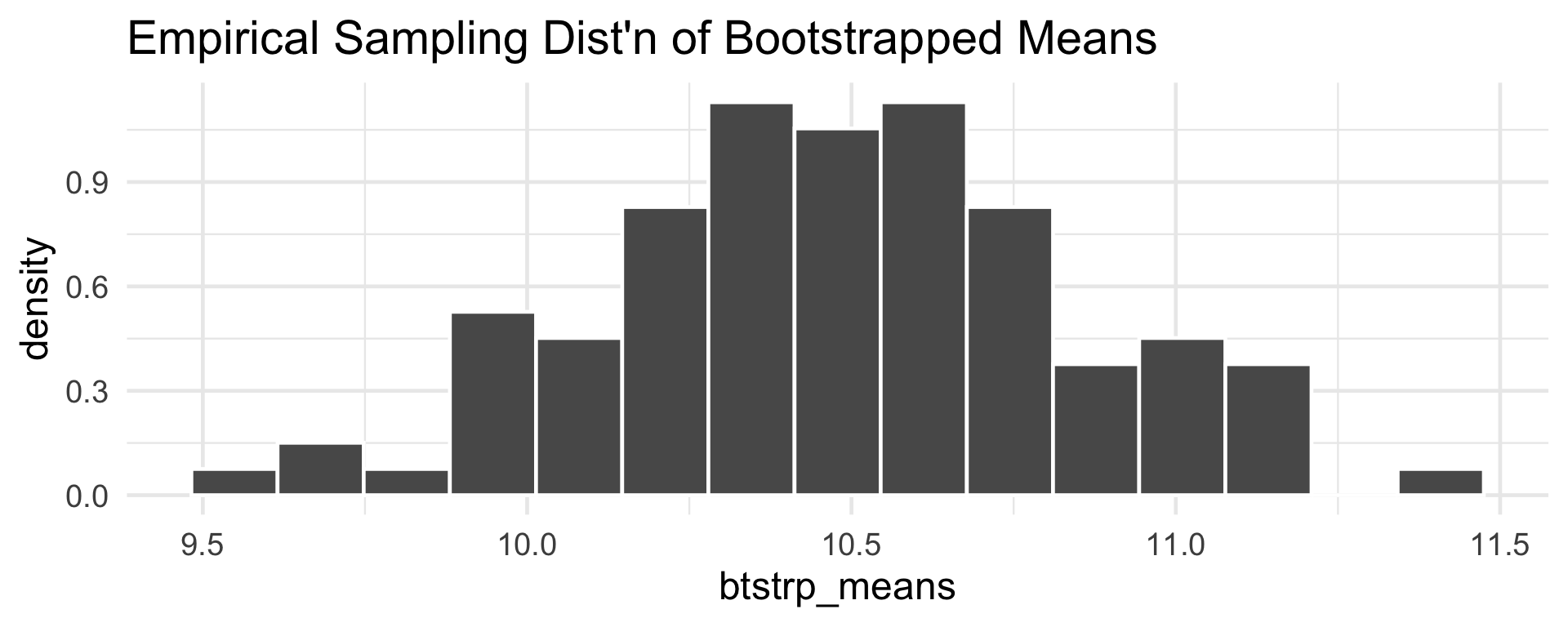
Bootstrapping: Example

• Since this data was simulated, we can actually assess how well the bootstrap is doing.

• Specifically (even though I did not tell you this before), the cat_wts vector was sampled from the \(\mathcal{N}(10.5, \ 3.2^2)\) distribution.

• So, let’s compare our bootstrapped sample means against a set of sample means drawn directly from the population distribution.

sm_from_pop <- c()
for(b in 1:1000){sm_from_pop <- c(sm_from_pop,
                                  rnorm(100, 10.5, 3.2) %>% mean())}

summary(sm_from_pop)

   Min. 1st Qu.  Median    Mean 3rd Qu.    Max. 
  9.285  10.276  10.493  10.499  10.711  11.482 

summary(btstrp_means)

   Min. 1st Qu.  Median    Mean 3rd Qu.    Max. 
  9.549  10.237  10.482  10.482  10.704  11.408 

Bootstrapping: Example

data.frame(`From Pop.` = sm_from_pop, 
           `Bootstrapped` = btstrp_means,
           check.names = F) %>%
  melt(variable.name = "type") %>%
  ggplot(aes(x = type, y = value)) +
  geom_boxplot(fill = "#dce7f7", staplewidth = 0.25,
               outlier.size = 2) + theme_minimal(base_size = 18) +
  ggtitle("Boxplot of Means", 
          subtitle = "Sampled from Population, and Bootstrapping")

Bootstrapping CIs

• What this means is that we can actually construct confidence intervals using bootstrapping.

• There are actually many different flavors of bootstrapped CIs; we’ll only discuss one in this class.

• Specifically, let’s go back to how I defined a confidence interval: an interval that we believe, with coverage probability, covers the true value of the parameter of interest.

• An equivalent way of interpreting a p CI is: if we were to repeat the mechanism used to generate the CI a large number of times, we would expect (on average) (p×100)% of the resulting CIs to cover the true value of µ.

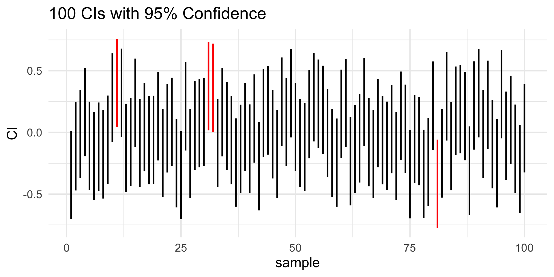
CI: Interpretation

Bootstrapping CIs

• “If we were to repeat […] large number of times”; isn’t that exactly what we do in the bootstrap?
  • Yup!
• So, here’s a way we can use the Bootstrap to obtain a p CI:
  1. Generate a large number of bootstrapped estimators
  2. Use the (1 - p)/2 and (1 + p)/2 quantiles of the bootstraped sampling distribution
• This has the benefit of being “distribution free” (sometimes called nonparametric), and can be used to construct confidence intervals for a wide array of parameters (not just the mean).