PSTAT 100: Lecture 09
Introduction to Inferential Statistics
Probability vs. Statistics
An Illustration
- Consider a bucket comprised of blue and gold marbles, and suppose we know how many blue and gold marbles there are.
- From this bucket, we take a sample of marbles.

- We then use our information of the configuration of marbles in the bucket to inform us about what’s in our hand.
- E.g. what’s the expected number of gold marbles in our hand?
- E.g. what’s the probability that we have more than 3 blue marbles in our hand?
Probability vs. Statistics
An Illustration
- Consider now the opposite scenario: we do not know anything about the configuration of marbles in the bucket. All we have is a sample of, say, 11 blue and 6 gold marbles drawn from this bucket.

- We then use our information on the configuration of marbles in our hand to inform us about what’s in the bucket.
- E.g. what’s the expected number of gold marbles in the bucket?
- E.g. what’s the probability that there are more than 3 blue marbles in the bucket?
Statistical Inference
General Framework
- Now, instead of marbles in a bucket, imagine units in our sampled population.
We have a population, governed by a set of population parameters that are unobserved (but that we’d like to make claims about).
To make claims about the population parameters, we take a sample.
We then use our sample to make inferences (i.e. claims) about the population parameters.

Cats!

Cats!

Cats!

Cats!

Sampling Distributions
Normal Example
Sampling Distributions
Normal Example
Sampling Distributions
Normal Example
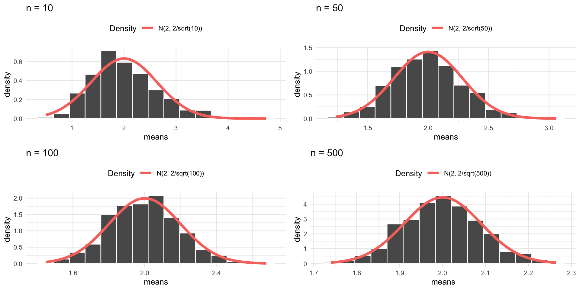
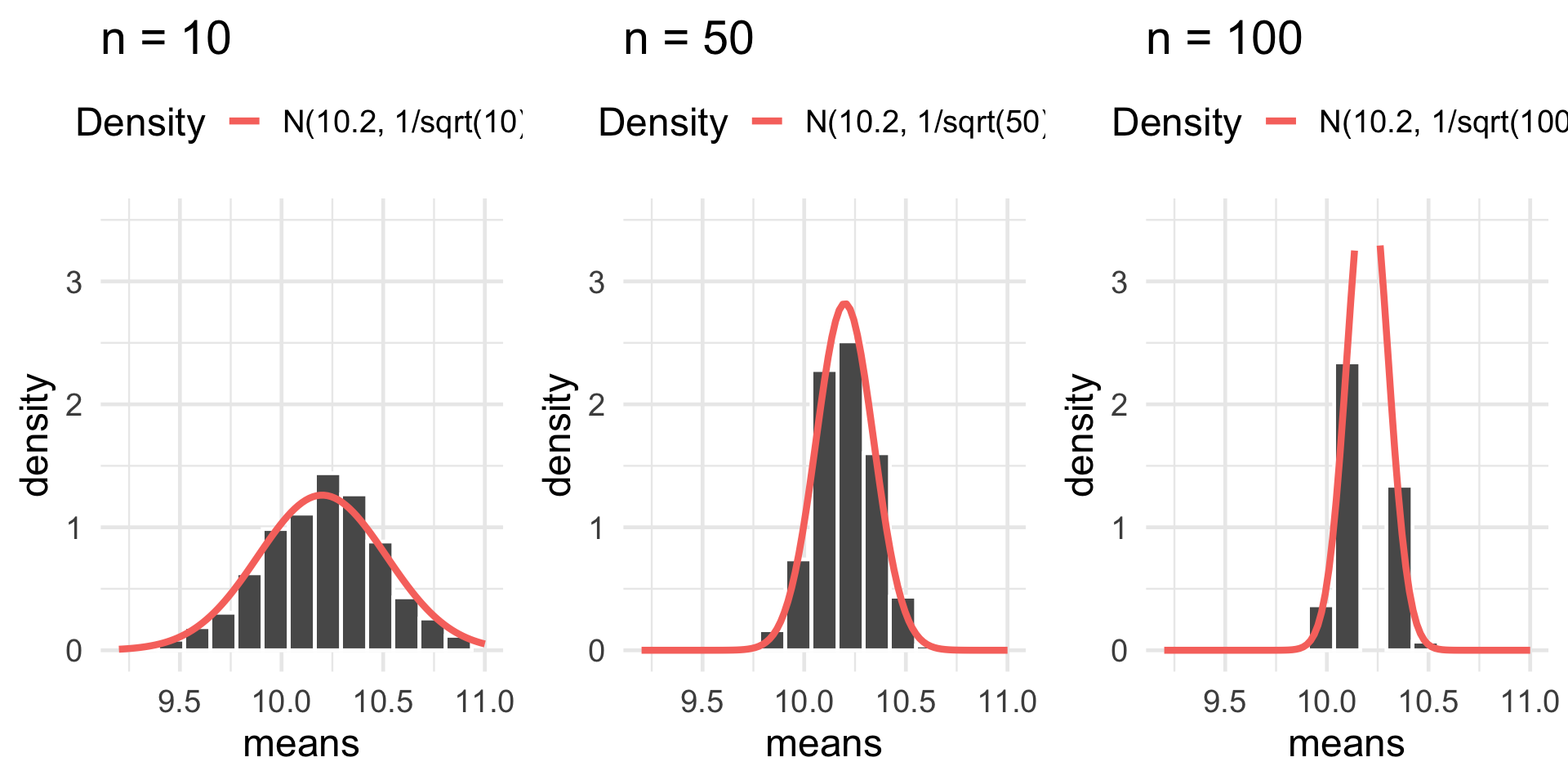
Sampling Distributions
Sample Mean: Normal Population
Proportions as Means
By the way, like we talked about in lecture yesterday, proportions are actually just a special case of means: specifically, a proportion is just a mean of binary 0/1 values.
As an example, imagine tossing a coin:

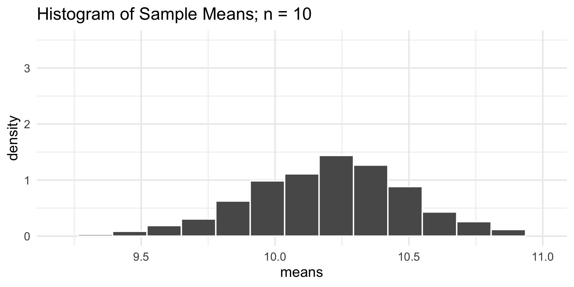
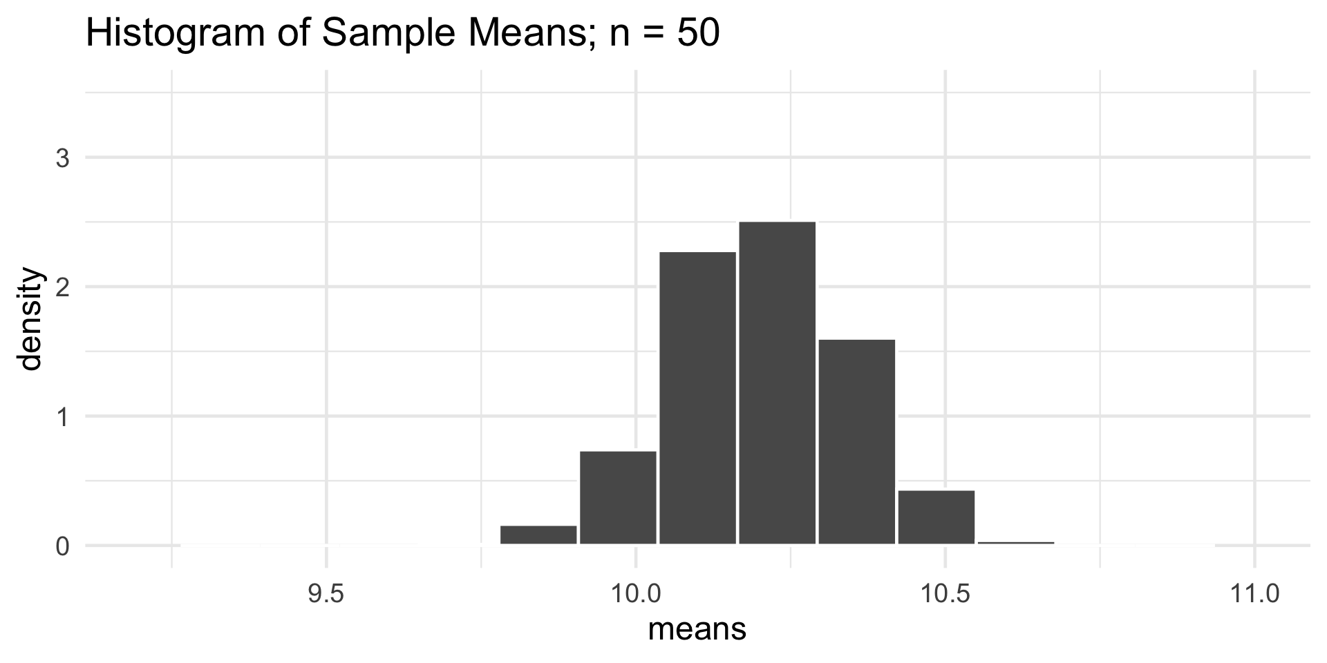
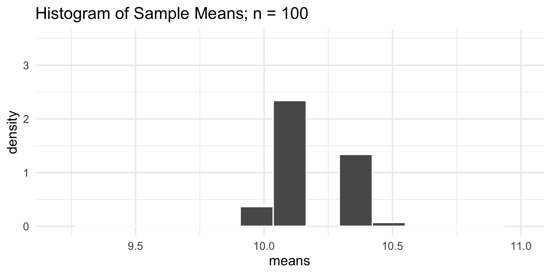
Sampling Distributions
Sample Mean: Non-Normal Population
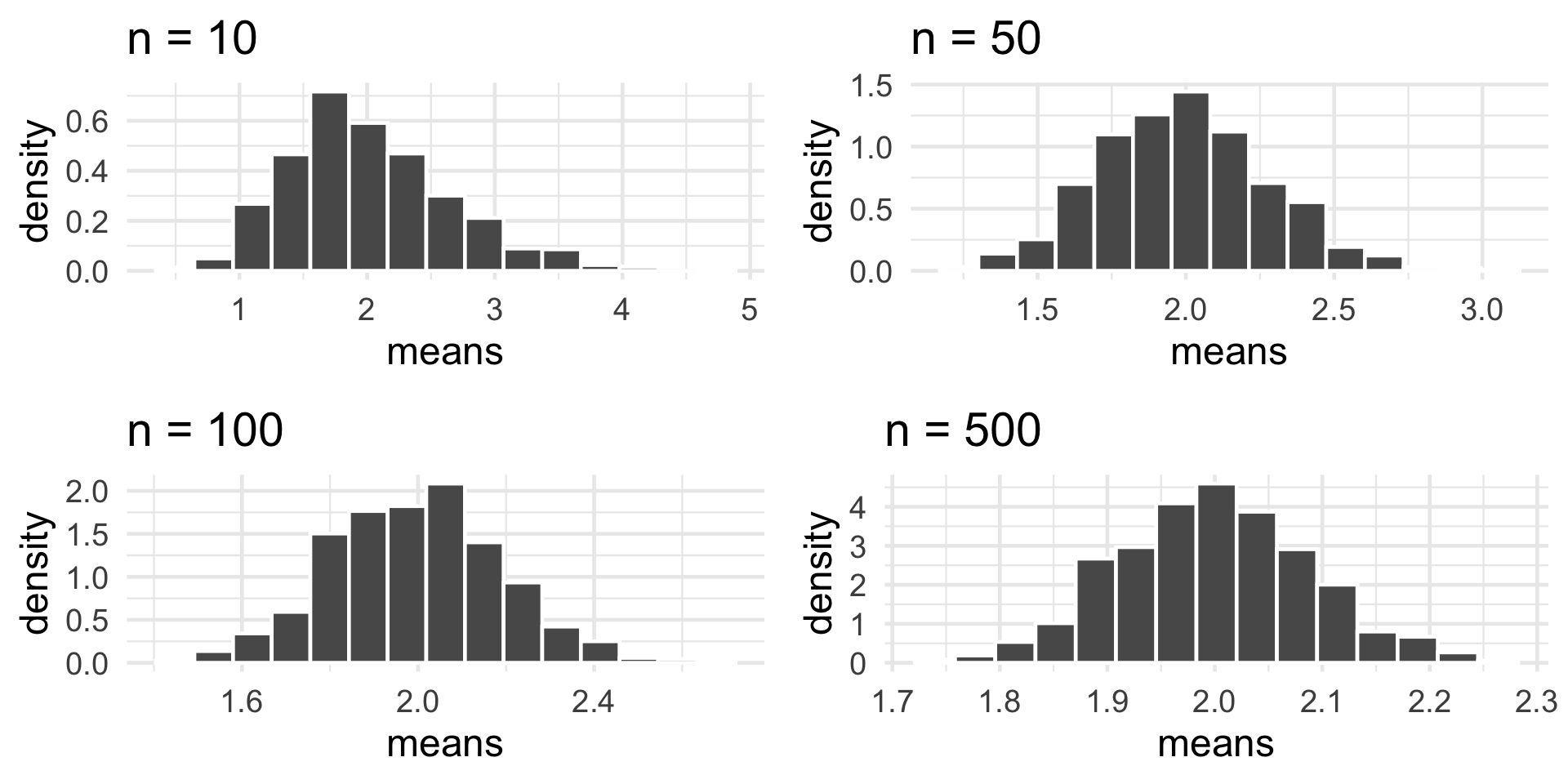
Sampling Distributions
Sample Mean: Non-Normal Population